ABSTRACT (original article): The mathematical constant π has traditionally been considered the circle constant. However, in recent decades, a growing body of mathematicians and educators has argued that 2π-the number of radians in a full turn-is a more natural and fundamental constant. This essay summarises the historical development of π, and presents the case for adopting the constant 2π. We demonstrate its implementation in the symbolic programming language Wolfram Mathematica. By implementing a custom constant for 2π, we aim to encourage its adoption and facilitate a clearer mathematical notation. CITATION (original article): Alberto Hijano, Implementing 2π as a custom constant in Mathematica, https://doi.org/10.13140/RG.2.2.21892.23685
Introduction
Introduction
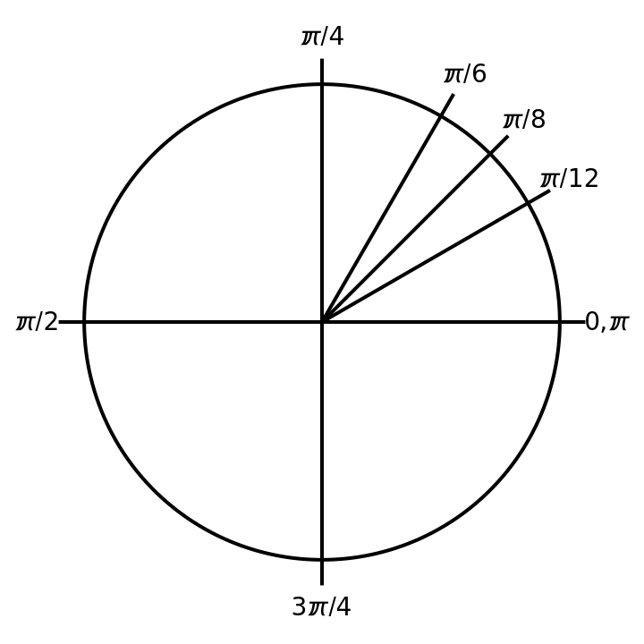
The mathematical constant π has long been regarded as the fundamental circle constant, yet a growing movement advocates for 2π—representing the number of radians in a full turn—as a more natural and pedagogically intuitive choice. This notebook explores the implementation of 2π as a custom constant (denoted here as , or “pipi”) in Wolfram Mathematica, demonstrating its seamless integration into symbolic and numerical computations. By redefining common formulas—such as those for circumference, area, angular frequency, and Fourier transforms—to use 2π directly, the notebook highlights how this approach simplifies mathematical expressions and aligns with geometric intuition. Custom formatting rules ensure readability, while practical examples in physics, such as calculating the decay rate of a scalar particle in quantum field theory, showcase its utility in real-world applications. The notebook also includes visualizations of trigonometric functions and angles on the unit circle, reinforcing the conceptual clarity of using 2π as the standard circle constant. This work aims to bridge theoretical advocacy with computational practice, offering a flexible framework for adopting 2π in education and research.
Definition of
Definition of
Symbolic
In[]:=
=2π;
Numeric
In[]:=
N[,20]
Out[]=
6.2831853071795864769
Custom output formatting
In[]:=
Unprotect[MakeBoxes];MakeBoxes[Times[n_,π],form_]:=Module[{m},m=n/2;If[m===1,RowBox[{""}],RowBox[{ToString[m,form]," ",""}]]];Protect[MakeBoxes];
In[]:=
2π
Out[]=
Basic relations
Basic relations
Geometric formulas
Geometric formulas
Circumference
C=r
Area of a circle
A=
1
2
2
r
Physical magnitudes and constants
Physical magnitudes and constants
Frequency
ω=f
ω=
T
Wavenumber
k=
λ
Reduced Planck constant
ℏ=
h
Complex analysis
Complex analysis
n-th roots of unity
z
k
k/n
Residue theorem
∮
C
∑
k
a
k
Distributions
Distributions
Dirac delta
δ(t-)=
t
0
∞
∫
-∞
ω
ω(t-)
t
0
Integral transforms
Integral transforms
Fourier series
F
k
1
T
T
∫
0
-kt/T
f(t)=
∞
∑
k=-∞
F
k
kt/T
Fourier transform
F(ω)=tf(t)
∞
∫
-∞
-ωt
f(t)=F(ω)
∞
∫
-∞
ω
ωt
Discrete-time Fourier series
F
k
1
N
N-1
∑
n=0
f
n
-kn/N
f
n
N-1
∑
k=0
F
k
kn/N
Discrete-time Fourier transform
F(ω)=Δt
∞
∑
n=-∞
f
n
-nωΔt
f
n
/Δt
∫
0
ω
nωΔt
Laplace transform
F(s)=tf(t)
∞
∫
0
-st
f(t)=F(s)
γ+∞
∫
γ-∞
s
st
Z-transform transform
F(z)=
∞
∑
n=0
f
n
-n
z
f(t)=F(z)
∮
C
z
n-1
z
Physical formulas
Physical formulas
Magnetic field around a wire
B=I
μ
0
r
Electric field of a point change
E=
q
2
ϵ
0
2
r
Identities
Identities
Euler’s identity
Euler’s identity
In[]:=
Out[]=
True
Periodicity of trigonometric functions
Periodicity of trigonometric functions
In[]:=
Sin[x+]==Sin[x]Cos[x+]==Cos[x]
Out[]=
True
Out[]=
True
Normal distribution
Normal distribution
In[]:=
1
-
2
x
2
Out[]=
True
Graphical showcase
Graphical showcase
Quadrants and special angles
Quadrants and special angles
In[]:=
θList={0,/12,/8,/6,/4,/2,3/4};labels={"0,","/12","/8","/6","/4","/2","3/4"};
In[]:=
xmax=1.3;rmax=1.1;rlabels=1.2;circumference={PolarPlot[1,{ϕ,0,},PlotStyle->Black]};radiuses=Table[ParametricPlot[{rCos[θList[[i]]],rSin[θList[[i]]]},{r,0,rmax},PlotStyle->Black],{i,1,Length[θList]}];
In[]:=
Show[Join[circumference,radiuses],PlotRange->{{-xmax,xmax},{-xmax,xmax}},Axes->False,Epilog->Table[Style[Text[labels[[i]],{rlabelsCos[θList[[i]]],rlabelsSin[θList[[i]]]}],14],{i,1,Length[labels]}]]
Out[]=
Trigonometric functions
Trigonometric functions
Practical example: Decay of a scalar particle
Practical example: Decay of a scalar particle
Consider the following Lagrangian, involving two real scalar fields Φ and ϕ:
Calculate the lifetime of Φ to lowest order in μ.
Solution:
Solution:
The decay rate of particle Φ in its rest frame is given by
The delta function can be rewritten as
and the radial integral is:
CITE THIS NOTEBOOK
CITE THIS NOTEBOOK
Implementing 2π as a custom constant in Mathematica
by Alberto Hijano
Wolfram Community, STAFF PICKS, June 30, 2025
https://community.wolfram.com/groups/-/m/t/3487366
by Alberto Hijano
Wolfram Community, STAFF PICKS, June 30, 2025
https://community.wolfram.com/groups/-/m/t/3487366