Find second part here: https://community.wolfram.com/groups/-/m/t/3345561
Abstract: The Schrödinger equation is central to quantum mechanics, describing the time evolution of wavefunctions in both analytical and numerical contexts. Bohmian mechanics extends this framework by providing a causal interpretation of quantum phenomena, linking the wavefunction to particle trajectories through the gradient of its phase or the quantum potential. This paper explores Fourier analysis as a fundamental tool for solving the Schrödinger equation, enabling transitions between momentum and position space to simplify differential equations. Part 1 introduces continuous Fourier methods, while Part 2 focuses on numerical solutions using the discrete Fourier transform (DFT). The DFT is particularly valuable in simulations, replacing computationally intensive numerical differentiation with efficient algebraic operations. Applications include one-, two-, and three-dimensional systems, emphasizing wavefunction superposition, interference, and particle scattering at potentials. Mathematica is employed as the computational framework for this investigation, leveraging its advanced Fourier capabilities to examine Bohmian trajectories and optimize wavefunction calculations.
Full list of posts: https://community.wolfram.com/web/kvbloh/
Note: see the detailed introduction to the de Broglie Bohm theory and implicit scheme method here:
https://community.wolfram.com/groups/-/m/t/3000266
https://community.wolfram.com/groups/-/m/t/3143785
https://community.wolfram.com/groups/-/m/t/3145353
https://community.wolfram.com/groups/-/m/t/3240209
1. Introduction
1. Introduction
Sometimes it is necessary to end a Wolfram Language kernel session or to clear all values, definitions, attributes, defaults, options and messages for the symbols.
In[]:=
Quit[]
In[]:=
ClearAll["Global`*"]
Use the following command, if you need to save/export graphs created by Mathematica into the current notebook directory:
In[]:=
SetDirectory[NotebookDirectory[]]
Out[]=
I:\Mathematica Notebooks
Feel free to use, reproduce, and modify this code in its entirety or in part of it. A further note: Some descriptions might be formulated too simply and could possibly require a more detailed explanation. I applied parallelization of the computational steps only in areas where a significant increase in processing speed could be achieved.
WARNING: These notes are incomplete and may contain errors in the implementation of the code and in the implementation of the equations. The essay has been written to the best of my knowledge and with great care. Every equation has been checked. It cannot be ruled out that errors may still exist. Some of the formulations are not introduced with mathematical precision and may contain linguistic inaccuracies. For simplicity, the SI units are not used at all. The author hopes, that readability is not significantly affected by this. The essay has not undergone a detailed peer review. Attention was paid to the clarity and comprehensibility of the equations. Therefore, many equations were not combined into a single expression. This sometimes results in less than optimal computational efficiency. They rather serve didactic purposes and aim to contribute to an understanding of numerical mathematics. Similarly, I have not indicated quotes from my own works. To the best of my knowledge, I have listed all individuals from whom I have adopted parts of the programs. If I have overlooked individuals who contributed to the algorithms employed, it is solely my responsibility.
WARNING: These notes are incomplete and may contain errors in the implementation of the code and in the implementation of the equations. The essay has been written to the best of my knowledge and with great care. Every equation has been checked. It cannot be ruled out that errors may still exist. Some of the formulations are not introduced with mathematical precision and may contain linguistic inaccuracies. For simplicity, the SI units are not used at all. The author hopes, that readability is not significantly affected by this. The essay has not undergone a detailed peer review. Attention was paid to the clarity and comprehensibility of the equations. Therefore, many equations were not combined into a single expression. This sometimes results in less than optimal computational efficiency. They rather serve didactic purposes and aim to contribute to an understanding of numerical mathematics. Similarly, I have not indicated quotes from my own works. To the best of my knowledge, I have listed all individuals from whom I have adopted parts of the programs. If I have overlooked individuals who contributed to the algorithms employed, it is solely my responsibility.
2. Introduction to the Fourier Series
2. Introduction to the Fourier Series
The Fourier series, developed by Joseph Fourier [19], an 18th-century French mathematician, is a mathematical tool that enables the representation of a periodic function as a sum of simple sine and cosine functions [17]. These fundamental oscillatory functions, often referred to as eigenfunctions in quantum mechanics, form a complete basis for describing periodic phenomena.
The Fourier series provides a framework to decompose such wavefunctions into their fundamental frequency components, with each component corresponding to a sine or cosine function of a specific frequency and amplitude. This decomposition is particularly valuable for analyzing complex wavefunctions, as it allows for a systematic study of their properties in terms of simpler, well-understood harmonic components.
This approach underscores the principle that any periodic wavefunction can be expressed with arbitrary precision as a linear combination of eigenfunctions, providing a powerful method for solving and interpreting quantum mechanical problems.
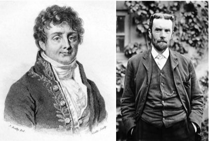
Figure 1. Joseph Fourier [19] and Oliver Heaviside[ 21] (images from [Wikipedia]).
The following calculation steps show some partial Fourier series results for the components of a square wave of length . The eigenfunctions form a normalized and orthogonal system (the example is taken from [2]). Orthogonality of eigenfunctions means that different eigenfunctions of an operator are orthogonal to each other, i.e. the integral over the entire space of two different eigenfunctions is zero.
L
ClearAll["Global`*"]phi[n_,x_]:=Sin[nPix/L]Print["Proof: normalization"]Simplify[Integrate[phi[k,x]*phi[k,x],{x,0,L}],Assumptions->{k}∈Integers]Print["Proof: integrate"]Integrate[phi[j,x]phi[k,x],{x,0,L}]//SimplifyPrint["Proof: 0 = orthogonal? "]Simplify[Integrate[phi[j,x]*phi[k,x],{x,0,L}],Assumptions->{j,k}∈Integers]
2
L
Proof: normalization
Out[]=
1
Proof: integrate
Out[]=
2kCos[kπ]Sin[jπ]-2jCos[jπ]Sin[kπ]
2
j
2
k
Proof: 0 = orthogonal?
Out[]=
0
This allows any continuous function over an interval to be approximated with arbitrary precision using a partial sum, where the Fourier coefficients converge to zero as . To keep the example simple, the Fourier series is computed for a constant over a given interval, here, with the constant . The interval is <=x<=. This step function is called the Heaviside function in mathematics. It is named after the British mathematician and physicist Oliver Heaviside (1850-1925) [22] .
n→∞
2
L
L
4
3L
4
The Fourier coefficients can be calculated by integrating the signal function multiplied by the corresponding eigenfunction over the given interval.
In[]:=
para={L->Pi};phi[n_,x_]:=Sin[nPix/L]psi[x_][nmax_]:=Sum[c[n]phi[n,x],{n,1,nmax,1}]signal[x_]=/.para;
2
L
2
L
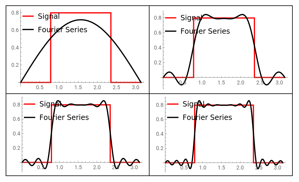
The coefficients, representing the amplitude of the corresponding sine waves, are calculated using the following integral. The Gibbs phenomenon[21] is the oscillatory behavior of the Fourier series of a piecewise continuously differentiable periodic function around a jump discontinuity, which is, here, clearly seen.
c[n_]=Integrate[signal[x]*phi[n,x],{x,L/4,3L/4}]//PowerExpand//Simplify;Print["Fourier coefficients:"]Table[c[n]/.para//PowerExpand//Simplify,{n,1,8}]fs=Table[psi[x][i]/.para,{i,1,32,1}];graphTable=GraphicsGrid[Partition[Table[Plot[{Piecewise[{{signal[x],L/4<x<3L/4}/.para}],fs[[i]]},{x,0,L/.para},PlotRange->Automatic,Axes->True,PlotStyle->{{Thick,Red},{Thick,Black}},PlotLegends->Placed[{"Signal","Fourier Series"},{Left,Top}]],{i,1,Length[fs],8}],2],FrameAll,ImageSize->500]ImageResize[graphTable,{640,480}];
Fourier coefficients:
Out[]=
,0,-,0,-,0,,0
2
2
π
2
2
3π
2
2
5π
2
2
7π
Out[]=
In[]:=
filename="Fourier1_Dec14.gif";directory="AnimationsFiles";Export[NotebookDirectory[]<>FileNameJoin[{directory,filename}],graphTable,RasterSize->1000,CompressionLevel->1];PictureGif=Import[NotebookDirectory[]<>FileNameJoin[{directory,filename}],ImageSize->800];
The graphs illustrate some partial Fourier series results for the components of a square wave. The Mathematica ‘built-in’ functions HeavisideTheta, FourierSeries and FourierCoefficient make it much easier. The absolute values of the complex Fourier coefficients converge to zero as .
n→∞
FourierSeries[HeavisideTheta[x],x,6]Table[FourierCoefficient[HeavisideTheta[x],x,i],{i,0,10,1}]Table[Abs[FourierCoefficient[HeavisideTheta[x],x,i]],{i,0,10,1}]
Out[]=
1
2
-x
π
x
π
-3x
3π
3x
3π
-5x
5π
5x
5π
Out[]=
,-,0,-,0,-,0,-,0,-,0
1
2
π
3π
5π
7π
9π
Out[]=
,,0,,0,,0,,0,,0
1
2
1
π
1
3π
1
5π
1
7π
1
9π
Here are a few examples of the Fourier series:
In[]:=
signallist={HeavisideTheta[x],Piecewise[{{-1/4,x<0},{1/4x,x>0}}],x/5,x^2Exp[-x^2]};Grid[Join[{{"Signals","Fourier Series"}},fs=Transpose[{signallist,Map[FourierSeries[#,x,5]&,signallist]}]],Background{None,{{None,GrayLevel[.9]}},{{1,1}Hue[.6,.4,1],{1,2}Hue[.6,.4,1]}},BaseStyle{FontFamilyTimes,FontSize10},DividersAll,FrameStyleHue[.6,.4,.8],Spacings{2,1}]//TraditionalForm
Here some plots:
3. Importance of the Fourier Transform for Analytical Solutions of the Schrodinger Equation
3. Importance of the Fourier Transform for Analytical Solutions of the Schrodinger Equation
4. From Position to Momentum: A Fourier Approach to the Schrödinger Equation’s Analytical Solution
4. From Position to Momentum: A Fourier Approach to the Schrödinger Equation’s Analytical Solution
4.1 An Example: The Free Particle for the One - And Two - Dimensional Case
4.1 An Example: The Free Particle for the One - And Two - Dimensional Case
4.1.1 The One - dimensional case for a Free Particle
4.1.1 The One - dimensional case for a Free Particle
The normalization factor, which is not important for the motion, could be calculated by:
4.1.2 The Two- dimensional case for a Free Particle
4.1.2 The Two- dimensional case for a Free Particle
The two-dimensional treatment of the free particle is the same as in the one-dimensional case.
The normalization factor, which is not important for the motion, could be calculated by:
4.1.3 Interference of Three Wave Packets
4.1.3 Interference of Three Wave Packets
The video below shows the temporal development of the wave densities.
IMPORTANT: Performance Warning
The creation of the ‘video frames’ can be very time-consuming due to the CPU capacity.
The creation of the ‘video frames’ can be very time-consuming due to the CPU capacity.
4.2 Various Solutions for the Free Particle via the Fourier Transform
4.2 Various Solutions for the Free Particle via the Fourier Transform
4.3 The Wavefunction in an Uniform Field
4.3 The Wavefunction in an Uniform Field
Using the following ansatz:
The above ordinary differential equation (ODE) is satisfied with the following ansatz.
Transformation into the positions-space leads to the unnormalized wavefunction for the one -dimensional case:
The normalization factor, which is not important for the motion, could be calculated by
IMPORTANT: Performance Warning
The creation of the ‘video frames’ can be very time-consuming due to the CPU capacity.
The creation of the ‘video frames’ can be very time-consuming due to the CPU capacity.
CITE THIS NOTEBOOK
CITE THIS NOTEBOOK
Solving the Schrödinger Equation 1: an introduction to Fourier analysis and application
by Klaus von Bloh
Wolfram Community, STAFF PICKS, December 16, 2024
https://community.wolfram.com/groups/-/m/t/3340354
by Klaus von Bloh
Wolfram Community, STAFF PICKS, December 16, 2024
https://community.wolfram.com/groups/-/m/t/3340354