Wolfram Cloud Document

This computational essay systematically explores finite state machine (FSM) strategies in the iterated Prisoner’s Dilemma through exhaustive enumeration and evolutionary algorithms. Analyzing all unique 2- and 3-state FSMs reveals that exploitative strategies consistently outperform the celebrated tit-for-tat, violating Axelrod’s “be nice” principle. However, evolutionary experiments with larger FSMs show cooperation can emerge and persist under various conditions. Comprehensive robustness testing identifies critical thresholds (such as a 5% error rate) where cooperation collapses, while also revealing remarkable resilience in other scenarios.

These findings suggest that multiple paths to stable strategies exist, enriching our understanding of strategic interaction beyond simple reciprocity.

Introduction

The Puzzle of Cooperation

In [2], Robert Axelrod and William Hamilton made a discovery that would reshape our understanding of cooperation. Through computer tournaments where strategies competed in the iterated Prisoner’s Dilemma, they demonstrated that a simple strategy called tit-for-tat consistently triumphed over more sophisticated approaches. This strategy, which starts by cooperating and then mirrors the opponent’s previous move, seemed to solve a fundamental puzzle: how can cooperation emerge among self-interested agents without central authority?

Payoff diagram of the Prisoner’s dilemma game. C stands for cooperate and D for defect.

In[]:=

MatrixGame[{{{3,3},{0,5}},{{5,0},{1,1}}},GameActionLabels->{{"C","D"},{"C","D"}}]["Dataset"]

Out[]=

The payoff matrix above describes the scores obtained by both players after choosing an action. For example, if both players cooperate, both receive 3 points. If one player cooperates and the other defects, the cooperator gets 0 points while the defector receives 5 points. If both players defect, they each receive 1 point.

In a tournament setting, the same game is played multiple times. For example, in Axelrod’s tournament, each match consisted of 200 rounds and each program played against every other program, as well as itself and a program that played randomly. The other programs were written by professional game theorists

Since the celebrated tournament, ongoing research has attempted to understand these types of games and which strategies emerge as winners (see, for example [1], for a series of works following Axelrod’s tournaments).

The Power of Exhaustive Enumeration

This project presents a systematic exploration of strategies that can be encoded as finite automata in repeated games. Rather than organizing yet another tournament with human-made strategies, we ask a more fundamental question: what strategies actually exist in the space of small finite state machines, and how do they perform against each other?

Following Stephen Wolfram’s computational approach of exhaustively exploring simple systems to uncover complex behaviors, we generate and analyze every possible finite state machine with 2 and 3 states. For 2-state machines, this means examining all 64 configurations, reduced to 50 unique strategies after removing isomorphic duplicates. For 3-state machines, we analyze 5,832 possibilities, filtered to 1778 non-trivial unique strategies.

This exhaustive approach reveals that when the complete strategy space is considered, exploitative strategies consistently outperform tit-for-tat and other reciprocal strategies. The dominant strategies violate Axelrod’s cardinal rule of “be nice” by defecting first, achieving superior performance through sophisticated exploitation patterns that human intuition failed to anticipate.

Beyond Simple Tournaments

Our investigation doesn’t stop at static tournaments. We extend the analysis through:

Evolutionary Dynamics: When exhaustive analysis becomes computationally intractable (beyond 3 states), we employ evolutionary algorithms to explore how strategies adapt and compete in larger state spaces.

Robustness Testing: We subject discovered strategies to comprehensive stress tests (introducing noise, temporal discounting, dynamic payoff regimes, and invasion scenarios) to understand when and how cooperation survives or collapses.

Phase Transitions: We identify critical thresholds where cooperative equilibria suddenly fail, such as the discovery that just 5% error rate can cause cooperation to completely tank.

Environmental Variations: We explore regime-switching environments that alternate between cooperation-favoring and defection-favoring conditions, revealing how strategies must balance exploitation with adaptability.

Why This Matters

The implications extend far beyond game theory into fundamental questions about strategic interaction in biological, economic, and social systems. If simple defection-biased strategies dominate when the full space is considered, why do we observe cooperation in nature? Our results reveal a nuanced picture: while exploitative strategies excel in exhaustive tournaments, our evolutionary experiments show that cooperation can and does emerge under many conditions. The discovery of multiple paths to stable strategies, from pure cooperation to sophisticated mixed approaches, suggests that the landscape of strategic interaction is richer than previously thought.

This computational essay documents our work during the 2025 edition of the Wolfram Summer School, going from exhaustive enumeration through evolutionary exploration, revealing both surprising discoveries and sobering limitations. While tit-for-tat-type strategies may not be the universal champion, our results show that cooperation remains achievable through various mechanisms. The fragility we observe (such as cooperation collapsing at certain noise thresholds) coexists with remarkable resilience in other conditions, painting a complex picture of how cooperation can emerge and persist in strategic interactions.

A Note on Model Selection

In the literature, it is frequent to use memory-n strategies or history-dependent strategies (see, for example,

[3]

). For a fixed n, a memory-n strategy is a map

{C,D}

↦{C,D}

. Any such map can be encoded in an FSM of at most

states. Similarly, any FSM with k states implements at most a memory-

(k-1)

strategy. However, FSMs have been used in the past to study the iterated Prisoner’s Dilemma and similar games

[4]

Finite State Machines (FSM) as Strategies

What is a Finite State Machine?

A finite state machine (FSM) is a mathematical model that describes a system which can exist in exactly one of a finite number of states at any given time. Think of it as a simple “memory device” that remembers where it is and decides what to do next based on its current state and the input it receives.

Consider a traffic light:

◼

States: Red, Yellow, Green.

◼

Input: Timer expiration.

◼

Behavior: Red → Green → Yellow → Red (cycles through states).

Or a vending machine:

◼

States: “Waiting for money”, “Has $1”, “Dispensing item”

◼

Inputs: “Insert coin”, “Select item”, “Take item”

◼

Behavior: Different inputs cause transitions between states

Anatomy of an FSM

Every finite state machine has four key components:

States: The finite set of conditions the machine can be in

Initial State: Where the machine starts

Transitions: Rules that say “if you’re in state X and receive input Y, go to state Z”

Actions/Outputs: What the machine does in each state (crucial for game theory)

Why FSMs Are Suitable for Game Strategies

In game theory, an FSM captures a player’s bounded memory strategy:

◼

States represent “memory” (what the player remembers about game history)

◼

Transitions represent “reactions” (how the player updates their memory based on opponent moves)

◼

Actions represent “decisions” (what the player actually does—cooperate/defect in each state).

This is psychologically plausible since real players have limited memory and use simple rules to decide how to play.

Encoding Strategies by FSMs

As mentioned above, we need to represent the following information:

◼

States (including an initial state, which could be deterministic or random)

◼

Actions or outputs based on the current state

◼

Transitions: given a state and opponent’s action at time N, what state will I be at time N+1?

Let’s show how this works in practice with a very simple yet effective strategy for 2-player, 2-action games like the Prisoner’s Dilemma: tit-for-tat. In short, this strategy can be summarized as follows: start cooperating, then mimic the opponent’s behavior from the last turn.

Tit-for-tat FSM representation as an Association:

In[]:=

titForTat=<|"States"->{1,2},"InitialState"->1,"Actions"-><|1->"C",2->"D"|>,"Transitions"-><|{1,"C"}->1,(*Staycooperativeifopponentcooperates*){1,"D"}->2,(*Switchtodefectionifopponentdefects*){2,"C"}->1,(*Returntocooperationifopponentcooperates*){2,"D"}->2(*Continuedefectingifopponentdefects*)|>|>;

We can visualize the strategy by looking at its graph representation:

In[]:=

visualizeFSM[titForTat,Small]

Out[]=

	Green = Cooperate
	Red = Defect
	Black border = Initial

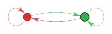
In this graph representation, nodes represent FSM states, with node colors indicating the action taken in each state (green for Cooperate, red for Defect). Edges show state transitions based on the opponent’s action, with edge colors matching the opponent’s move that triggers the transition (green edges for opponent cooperation, red for opponent defection). The initial state is marked with a thick black border. This visualization encodes the complete strategy: how the FSM responds to different opponent behaviors through state transitions and the action associated with each state.

Removing redundancies and counting unique strategies

How many distinct FSM strategies are possible? By simply counting all possible states, actions and transitions, one can in principle enumerate all FSM with a given number of states:

Displaying total number of FSM and their base 10 logarithm:

Out[]//TableForm=

States	Total FSMs	Log10(FSMs)
1	2	0.30103
2	64	1.80618
3	5832	3.76582
4	1048576	6.0206
5	312500000	8.49485
6	139314069504	11.144

As the table shows, the number of FSMs grows exponentially, and already for

k≥4

the number of tournament matches becomes unfeasible to compute. However, there is a lot of redundancy. To illustrate this, let’s look at two FSMs that are technically different but in practice are not:

Two different FSMs that have the same canonical representation:

In[]:=

fsm1=<|"States"->{1,2},"InitialState"->1,"Actions"-><|1->"C",2->"C"|>,"Transitions"-><|{1,"C"}->1,{1,"D"}->1,{2,"C"}->1,{2,"D"}->1|>|>;

In[]:=

fsm2=<|"States"->{1,2},"InitialState"->1,"Actions"-><|1->"C",2->"D"|>,"Transitions"-><|{1,"C"}->1,{1,"D"}->1,{2,"C"}->1,{2,"D"}->1|>|>;

Visualize them:

In[]:=

visualizeFSM[{fsm1,fsm2},Small]

Out[]=

	Green = Cooperate
	Red = Defect
	Black border = Initial

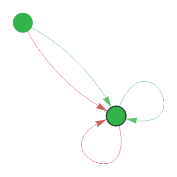
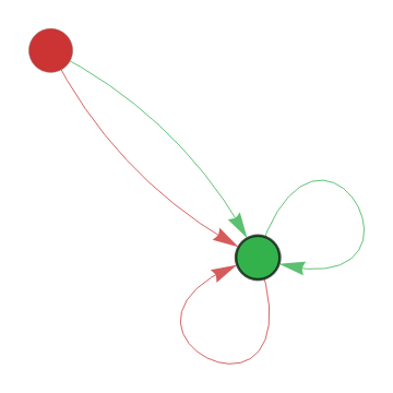
The reason both are equivalent is that they both get stuck forever in the initial green state. It doesn’t matter what you put outside since it won’t be reached.

The Canonical Form Algorithm

The Canonical Form Algorithm works as follows:

Start from the initial state and assign it number 1

Use breadth-first search (BFS) to explore reachable states

Assign new numbers to states in the order they’re discovered

Record both the actions and transitions in this new numbering

Create a unique string representation of the FSM structure

In the example above, both FSMs have the representation “{1,C,1,C,1,1,D,1}.” To see why, note that we assign number 1 to the initial state and record the “C” action. This yields {1,C} in the string representation. Then we record both transitions: {1,C,1} and {1,D,1}. Combine them gives us {1,C,1,C,1,1,D,1}. Since there are no more reachable states, the algorithm ends.

In the Appendix, you can find the implementation of the canonical form algorithm. To illustrate the impact of this algorithm, let’s see how they 3-state FSM space gets reduced by applying it:

Analyze 3-state FSM equivalence classes :

Reduction factor

When analyzing 2- and 3-state FSM tournaments, we’ll first apply the algorithm to consider only “unique” strategies. The latter is in quotes because even when considering equivalence classes, there are still behaviorally equivalent strategies despite having different structures.

Tournament Setup Outline

We now proceed to describe how we’ll set up the tournaments. There are two main categories of setups we’ll consider.

For 2- and 3-state FSMs, we’ll do an exhaustive analysis since it’s not very expensive to generate all possible FSMs. The tournament setting is a round-robin tournament, where all strategies play against each other (except themselves) in an iterated Prisoner’s Dilemma game for 50 rounds. Scores are accumulated over the rounds. At the end, we’ll analyze the results and see which strategies are the most effective.

◼

We’ll sample 1,000 strategies at random from all possible FSMs with 2-5 states (250 from each). This is our initial population.

◼

In the first generation, each strategy plays against 100 other strategies in an iterated Prisoner’s Dilemma game for 50 rounds.

◼

We resample from the population proportionally to the scores obtained in the previous round (see this link for details).

◼

With a certain probability, some strategies will mutate (i.e., add or remove a state, swap the action in a given state, or change a transition).

◼

Repeat for 1000 generations.

We then proceed to examine statistics such as the mean payoff per generation, the cooperation rate on the first move, and the top performers at the end. Since each experiment takes around 15 minutes on my machine, we’ll show the final results and code to replicate the experiments (since this involves random variables, we also provide the seed used).

After performing this baseline experiment, we’ll consider several variations to see whether the behavior changes. These include:

◼

Increasing the mutation rate

◼

Adding a random noise to the actions (with a certain probability, players will choose the opposite action “by accident”)

◼

Adding a discount rate to the payoffs (so that future payoffs are worth less than current onces)

◼

Considering dynamic payoffs, where we use two or more payoff matrices so that at each time, one of them is chosen (either in a deterministic cycle, a Markov chain, or a hybrid regime)

◼

Adding invasions: starting from a baseline population, we replace a fraction of the population with “invader strategies” to see whether that alters the population mix.

We test each of these in isolation first, then mix two of them, and finally include them all.

2- and 3-state FSM Tournaments

2-State Tournament

Create and visualize 10 FSMs with 2 states:

We note something from looking at these strategies. There are at least two strategies that are “cooperate-only” and “defect-only.” In principle, these FSMs are not unique since they have different transitions, but they are behaviorally equivalent. Since it is easy to detect these strategies, we’ll only consider one of each for the tournament:

Compare size of strategy space before and after removing cooperate-only and defect-only strategies:

Number of unique strategies after removing cooperate-only and defect-only strategies:

Now, we’ll run the tournament over the 27 unique strategies after removing all but one cooperate-only and defect-only strategies.

Display ranking of strategies for 50-round tournament with frames

Let’s visualize the top-10 strategies:

Let’s describe in words what each strategy does:

◼

FSM #10 is called a “grim trigger” strategy. It starts cooperating and continues doing so until the opponent defects. From there on, it defects forever.

◼

FSMs #2 and #3 are defect-only strategies. Even though FSM #2 has a cooperative state, it is unreachable, so it is a de facto defect-only strategy.

◼

FSM #26 only cooperates on the first turn and then it defects forever. It is a slight variation of the previous two strategies.

◼

FSM #5 starts defecting and continues doing so while the opponent cooperates. Once the opponent defects, it cooperates for one turn and goes back to defecting.

◼

FSM #9 starts defecting and continues doing so while the opponent cooperates. Once the opponent defects, it cooperates while the opponent does so. If the opponent defects, then it goes back to defecting as at the start.

◼

FSM #7 starts defecting and continues doing so while the opponent cooperates. Once the opponent defects, it starts cooperating and continues doing so while the opponent defects (!!). If the opponent cooperates, then it goes back to defecting as at the start.

◼

FSM #24 starts cooperating and then switches to defecting no matter what the opponent does. It continues defecting while the opponent cooperates, and then switches to cooperating for one turn once the opponent defects.

◼

FSM #8 starts cooperating and continues doing so while the opponent cooperates. Whenever the opponent defects, it switches action and continues doing the same action while the opponent cooperates.

◼

FSM #6 is the tit-for-tat strategy.

Overall, we see mostly exploitative strategies at the top, with tit-for-tat having a ranking of 10/27.

3-State Tournament

We proceed to do the same analysis for 3-states FSMs.

Create and visualize 10 FSMs with 3 states:

Filter by cooperate-only and defect-only strategies:

Number of unique strategies after removing cooperate-only and defect-only strategies:

Run tournament with filtered 3-state FSMs:

Display top 50 ranking of strategies for 50-round tournament with frames

Visualize top-10 strategies

We could again describe them in detail, but it starts to get tedious and a picture can be more descriptive. Nevertheless, we can capture some patterns:

◼

All start defecting and continue doing so while the opponent cooperates

◼

All have 2 defecting states and 1 cooperative state

◼

Most require the machine to visit state 2 (also D) before it can reach the cooperative state 3.

◼

Duration of the cooperative state is only one turn for all but FSM #51, which cooperates while the opponent also cooperates.

In summary, they all explore small variations on when they apologize, how long they remain kind, and how quickly they harden again.

Now that we have more FSMs, let’s also visualize a histogram of the scores:

Histogram of 3-state FSMs scores after tournament.

Beyond 3 states: Evolutionary Strategies

As we’ve already mentioned, extending the analysis for 4 and larger states becomes exponentially slower. Also, the previous analysis was static by definition since we only need to run the tournament once. However, in principle the number of strategies is infinite and players tend to adapt to the landscape, often by necessity. Just to give a simple example, if our “game” consists of buying and selling stocks, then a momentum trader will “follow the wave” and exit right before a shift occurs. A contrarian trader, on the other hand, may decide to buy when prices are dropping and sell otherwise. But the variety of strategies is endless and constantly evolving (this is why any strategy that seems to work stops doing so after it’s discovered by a significant number of people).

We’ll try to emulate this process in our simple Prisoner’s Dilemma game as described in the outline. See also the Appendix for the full code in case you want to run your own experiments.

Baseline Case

We start by analyzing the baseline case, where we only introduce mutations. The mutation rate is 2% (meaning that roughly 2% of the population suffers a mutation in each generation). I’ve tried different mutation rates (2%, 5%, and 10%) and the results were very similar (higher mutation rates increase the variance slightly). Thus, we only show the graphs for the 2% mutation rate. We show graphics regarding the evolution of average fitness, the first-move cooperation rate and the average complexity measured by number of states.

Blue plot: average fitness over time. Red plot: first-move cooperation rate over time. Green plot: average number of states over time.

We see that the first two graphs are highly correlated and, after an initial drop, the population tends to converge to strategies that always start cooperating. Let’s now take a closer look at the final generation by looking at its histogram and top-9 performers.

Histogram of fitness for the baseline case:

We can see from the histogram that the scores are highly concentrated around 140. To put things in context, a score of 150 is obtained by pure cooperation. The red graph and the histogram show that almost all strategies have a cooperation loop, so that it doesn’t matter much what do you do outside of this loop. For example, we see in position 6 a cooperate-only strategy, whereas position 9 is the grim-trigger strategy.

Visualization of top 9 performers. We used the canonical representation to avoid disconnected subgraphs:

Adding Noise

The idea behind this variation is that, with a fixed probability, the action taken will be the opposite of the one given by the state. Namely, if the action corresponding to the state is to cooperate, then the player defects (and vice versa). Adding noise can punish more rigid strategies like grim trigger. On the other hand, it can help exit defect loops to reach a more cooperative state. For example, if two tit-for-tat-type strategies get to a defection loop, having either of them mistakenly cooperate will lead the other to cooperate too.

I tested different configurations, and below I show the results for error rates of 3%, 4%, 5%, and 10% where all had a 2% mutation rate.

3% Noise Rate Plots

It’s interesting to see in this example that the first-move cooperation tanks to almost 0 (only 1 of the top 9 performers starts cooperating). Nevertheless, the scores remain very close to the baseline case. It seems, then, that adding a little bit of noise can open up different strategies.

Top-9 performers when adding a 3% noise:

Histogram of fitness when adding a 3% noise:

4% Noise Rate Plots

Here, scores also remain fairly stable and initial cooperation seems to emerge again.:

Top-9 performers when adding a 4% noise:

We start to see here more spreading of the scores:

5% Noise Rate Plots

Both the blue and red plot drop to pure defection levels:

Here we see something very interesting: scores tank together with the first-move cooperation! It seems this population gets stuck in a never-ending cycle of defection. The plot of top performers is also very eloquent: all strategies in the top 9 are defect-only (note that here we are not restricting to one strategy per equivalence class, so there can be repeated strategies as the visualization below shows). Also, recall that the reason the scores are slightly different is because each strategy competes with 100 other strategies, so there can be small variations.

The histogram shows the scores are highly concentrated around 60:

10% Noise Rate Plots

Just to make sure that 5% wasn’t a coincidence, I tried also with 10% noise rate:

Here the pattern is very similar to the 5% error rate, where basically the same behavior repeats.

The histogram is also highly concentrated, although the scores are slightly higher:

By performing several experiments, it seems that 5% is the critical rate at which the population collapses to a pure-defection spiral. In a sense, the 2% mutation rate is too weak to overcome the pressure from pure defectors. So what happens if we increase the mutation rate?

5% Noise Rate Plots + 3% Mutation Rate

It worked! By increasing the mutation rate, we created the possibility of developing a critical mass of different strategies. However, it’s not yet clear from the graphs whether the population will revert to a defection spiral or stabilize to a more cooperative state.

The histogram also shows more dispersion in the scores, so the system hasn’t yet converged to a steady state.

In any case, it seems that there is a phase transition for either end of the spectrum (cooperation vs. defection) depending on the mutation rate. In this example, for a 2% mutation rate, the threshold is at 5% error rate. I’m not aware whether this result has been proved elsewhere.

Adding Discount Rates to Payoffs

The next variation to our baseline case is adding a discount rate to the payoffs. The motivation here is very clear from a financial point of view for example: the time value of money. In other words, a dollar today is more valuable than a dollar one year from now. Alternatively, one can see it from a consumption point of view: I’d rather buy something today than in one year. A third view is that of uncertainty: an investment that pays me 100 dollars tomorrow is more valued than one that pays the same 100 dollars in 1 year (other things being equal) since many things can occur in one year.

I tested using discount rates of 0.99, 0.95, 0.9, and 0.8 (all with a mutation rate of 2%).

Discount rate of 0.99

Discount rate of 0.95

To put things into context, the seemingly low score of 50 for the mean is actually very close to the score obtained by a pure cooperation strategy (3 points discounted by 0.95 over 50 turns is around 55.38). However, with discounting it gets trickier to determine this optimal score due to the non-linear nature of the payoffs. In a sense, defecting early to try to get the 5 points may be a good idea, although we’ll see next that this is not always so clear.

Discount rate of 0.90

Again, the “optimal” score from discounting a pure-cooperation game is around 30, so this is very close to it. Also, it’s interesting to see a shift back to cooperation. Discounting adds a layer of non-linearity that may create different possibilities for reaching an optimal average score. In this case in particular, it seems that basically the whole population starts cooperating and keeps doing so while the opponent cooperates, so the rest of the configuration doesn’t matter much. Also, we remind the reader that the reason why strategies that are the same (like tit-for-tat or cooperate-only) appear in different rankings is because each strategy competes with 100 other strategies, so there can be a slight variation. In any case, in this particular example, the variation is minimal as we can see in the histogram below (the overwhelming majority has a score between 28 and 30, suggesting a cooperation-only loop).

Despite the fact that almost all the strategies start defecting, there is a whole variety of strategies regarding what’s done next. Again, we see the scores are highly concentrated around the mean.

Invasion robustness

The next experiment was fairly simple: we first ran a baseline population (as above) with only a 2% mutation rate for 500 generations. Then, we replaced a fixed percentage of the last generation with a population of 1-state, defect-only strategies. We then show the results of running the experiments for 1000 generation. Even after replacing the population with 90% defect-only FSMs, the population recovered very quickly to a cooperative state. This shows that the population is resistant to defect-only play (like tit-for-tat-type strategies) and since there is still a critical mass of cooperative FSMs, they end up scoring more points in a tournament. I didn’t try to add more sophisticated strategies, however, due to lack of time.

An interesting experiment would be the following: given a population, generate a subpopulation of invaders that performs, let’s say, at least 10% better than the average score and see what happens.

90% of defect-only invaders

Interestingly enough, in this round there are both cooperate-only and defect-only strategies!

Regime-Switching Payoffs

The next experiment consists of using more than one payoff matrix and sample from each of them at a time. The sampling can be deterministic (in a cyclical way), stochastic (Markov chain), or hybrid (deterministic cycle with a random chance of a shock that changes the payoff matrix). In all the tests, we considered two payoff matrices representing “Abundance” and “Scarcity.”

Payoff matrix in the Abundance case

Payoff matrix in the Scarcity case

In the experiments made, the transitions occurred between generations. An alternative experiment is to make the transitions between individual rounds.

Deterministic Cycle

In this case, we start with the abundance payoff and cycle between the two every 100 generations. The results are unsurprisingly cyclical

The score distribution is also highly concentrated:

From the data, we see that all leading strategies start cooperating and remain there no matter what. When there is a switch in regime, there is no adaptation and first-move cooperation remains high during most of the simulation. However, a jump under this model will be inevitable since the payoff structure under Abundance is higher than under Scarcity.

Stochastic Regime Switching

In this case, we start in the Abundance regime. Before starting a new generation, there is a 10% chance of switching to the opposite regime (either from Abundance to Scarcity or vice versa).

As we see from the pictures, typically there is a transition every 10 rounds. Again, we don’t see much difference in the first-move cooperation rate and a highly oscillatory pattern in the payoffs.

Hybrid Regime Switching

In this case, we run a cycle as in the first case, but on each generation there is a 5% chance that the regime switches.

Adding Two Variations

Now that we have analyzed individual variations, we’ll also consider some mixed variation and see whether the behavior changes compared to the baseline case and the individual variations. There are 6 possible variations, but to avoid making the essay too long, we’ll try 4 variations. Also, we’ll limit ourselves to trying a couple of parameters for each combination.
Unless indicated otherwise, all experiments have a mutation rate of 2%.

Putting It All Together

The final series of experiments we try is to combine all the stressors together. We test 3 variations:

◼

Low stress regime: 5% noise rate, 0.95 discount rate, and deterministic regime switching.

◼

Medium stress regime: 10% noise rate, 0.9 discount rate, and stochastic regime switching (with a 15% chance of switching state).

◼

High stress regime: 15% noise rate, 0.85 discount rate, and hybrid regime switching (with a 10% chance of switching state on top of the cycle).

In all experiments we used a 2% mutation rate. After that, we introduced different invasion rates. They didn’t make much of a difference, so we omit them from the analysis.

Conclusions

The battery of experiments conducted can be used as a guide for researching a large number of interesting problems. The main insights are as follows:

◼

When considering exhaustive tournaments over all FSMs with a given number of states, exploitative strategies tend to perform well since there are many naive strategies. Adding more states enables more nuanced strategies that can also profit from tougher opponents like tit-for-tat.

◼

The landscape appears different when considering evolutionary games over sampled populations.

◼

In general, what constitutes a good strategy depends heavily on the population. There is no bulletproof strategy that works well under all circumstances.

◼

In simple cases such as our baseline scenario, a cooperation loop seems to prevail regardless of initial conditions. This assumes a non-zero mutation rate to avoid the defection loop present in early generations.

◼

As soon as variations are introduced, the scenario becomes less clear.

◼

For instance, when adding 3% noise, the proportion of first-move cooperation plummeted, yet scores remained high. However, if noise is too large relative to the mutation rate, collapse into defection loops occurs. In our experiments, 5% noise was the critical threshold. This can be reversed by increasing the mutation rate.

◼

Discounting adds an interesting layer of non-linearity that seems to lead to multiple optimal strategies. In our experiments, scenarios with both high and low first-move cooperation rates achieved similar scores.

◼

Adding invaders to an already stable population doesn’t seem to affect long-term outcomes. However, adding invaders each generation may produce different outcomes. Similarly, introducing more capable invaders may create additional dynamics not seen in our experiments.

◼

Adding regime-switching payoff matrices alone didn’t change the cooperation structure and led to oscillatory mean payoff evolution. I suspect this depends heavily on the matrices themselves. It would be interesting to analyze whether the same behavior prevails when allowing payoff matrix transitions after every round instead of every generation. This may force more rapid adaptation. When transitions occur only at the generation level, there is no way to adapt mid-round, and equilibrium may take much longer to achieve.

◼

Higher mutation rates can help break defection loops by creating a larger critical mass of alternative strategies.

◼

In simpler scenarios, mean payoffs correlate directly with first-move cooperation rates. As more complexity is added, there are multiple paths to near-optimal mean payoffs.

◼

In some examples, phase changes took several hundred generations. Even 1000 generations may not be sufficient in some cases.

◼

As the example 0.90 Discount Rate + Stochastic Regime Switching showed, cooperation can also decline after long periods. Thus, even equilibria observed after 1000 steps may not be permanent.

◼

Generally, for simple scenarios, few states can perform as well as more complex ones. For complex scenarios, more states seem to provide greater benefits.

Future Work

Several experiments merit exploration after the Summer School. Just to mention a few:

◼

Prove or find a counterexample to the hypothesis that first-move cooperation rate approaches 1 as generations approach infinity. Since mutation can always flip initial state actions, the limit shouldn’t be 1 but should depend on mutation rate.

◼

Try different games as baselines and repeat the experiments.

◼

For a given population, find at least one strategy that outperforms the average payoff by 10%.

◼

Is this strategy robust under mutations? If so, one can then find multiple strategies by mutating the base strategy.

◼

Is the population resistant to such invaders? Is there a critical mass that causes evolutionary collapse?

◼

What happens if this procedure is repeated? Does it create a “super” strategy or converge to pure cooperation or defection?

◼

Try different tournament types.

◼

Run tournaments until the first player reaches a given score (e.g., 100 points), then perform fitness selection based on those scores.

◼

Instead of cumulative scores, assign 1 point to match winners after 50 rounds, 0 to losers, and split points for draws.

◼

Consider dynamic payoffs that depend on player actions. For example, in stock market games, payoffs depend on stock prices, which depend on supply and demand (number of buyers vs. sellers).

◼

What if players were meta-FSMs that pick between different strategies based on outcomes? How does this compare to having larger FSMs?

Appendix: Code

Acknowledgments

I would like to express my gratitude to the Wolfram Summer School Staff for making this transformative 3-week experience a reality. My sincere thanks go to my mentors Paul Abbott and Piero Sanchez for their invaluable guidance and feedback throughout the project, and to Zsombor Méder for his insightful remarks, comments, and relevant references that significantly enriched this work. I am grateful to Luzie Kupffer for her careful proofreading and thoughtful recommendations. Finally, I extend special thanks to Stephen Wolfram for selecting this project and sharing his valuable entrepreneurial insights.

References

Axelrod, R., & Dion, D. (1988). The further evolution of cooperation. Science, 242(4884), 1385-1390.

Axelrod, R., & Hamilton, W. D. (1981). The evolution of cooperation. Science, 211(4489), 1390-1396.

Hilbe, C., Martinez-Vaquero, L. A., Chatterjee, K., & Nowak, M. A. (2017). Memory-n strategies of direct reciprocity. Proceedings of the National Academy of Sciences, 114(18), 4715-4720.

Marks, R. E. (1990). Repeated games and finite automata. Sydney, Australia: Australian Graduate School of Management, University of New South Wales.

Cite This Notebook

Strategic Machines: Exhaustive Analysis of Finite State Automata in Games
by Rodrigo Bazaes
Wolfram Community, STAFF PICKS, July 9, 2025
https://community.wolfram.com/groups/-/m/t/3496890