Wolfram Cloud Document

ABSTRACT (original article): Detections of gravitational waves since GW150914 has gained a contemporary interest in potential quantum-classical correspondences between GWs and hypothetical gravitons. One such correspondence theory is stochastic gravity, whereby graviton fluctuations are treated as the stochastic noise embedded in global manifolds and local gravitational interactions. Utilizing the Einstein-Langevin equation that describes graviton fluctuations, in attempt to form a correlation with GW generation, we utilize the hollow mass shell model of coalescing compact binaries. This is to explore the second Newtonian postulate of neutralized internal gravitational fields, i.e., the stochastic noise of an enclosed, internal Minkowski manifold. This stochastic picture of GW formation implies the treatment of the enclosed gravitons as though it were a thermal Brownian bath. From the Einstein-Langevin equation, we establish a scaling relation where quanta dissipation depends inversely with the contracting volume (i.e., coalescence). Using an Euler iteration scheme, we simulate the graviton fluctuations from inspiral to merger as a Wiener process, revealing a signal that qualitatively resembles macroscopic GW waveforms. While inherently heuristic, this approach provides a computational framework for exploring graviton-scale perturbations in GW formation.
CITATION (original article): N. M. MacKay (in progress), Gravitational Wave Generation via the Einstein-Langevin Equation, arXiv:2410.04562. https://doi.org/10.48550/arXiv.2410.04562

Introduction

Gravitational waves are visualized as geometric ripples of the spacetime continuum, which are modeled intricately using analytical, effective-one-body wavefunctions, and numerical relativistic waveform models. If we adopt the stochastic gravity picture, such that these ripples are “quantized” as Brownian gravitons, we can treat the dynamics of coalescing binaries as a thermal gas model. Thermal gases follow a random walk classically described by the Langevin equation. For a stochastic gravity picture, the random walk of gravitons is mapped by the Einstein-Langevin equation. Much like the classically-framed Langevin equation, the general relativistic counterpart for metric fluctuations can be discretized and computationally simulated as an Euler scheme.

Insight to the Einstein-Langevin Equation

While we may observe gravitational waves being formed, and thus we can measure the elapsed time as the observer time, the Einstein-Langevin equation is a conformal time-dependent equation. The transformation between observer (t) and conformal (τ, in other literature η) times relies on the Friedmann-Walker picture of cosmology and the scalar factor a(τ). Note that the original application of the Einstein-Langevin equation is to the observable universe, hence the presence of a Hubble parameter in the final derivation in Ref. (https://journals.aps.org/prd/abstract/10.1103/PhysRevD.51.1577). However, to apply this to gravitons between two inspiraling masses, we apply a conformal picture of sizes, where globally flat and locally flat spacetimes are indistinguishable. This applies only if the spacetime we consider is flat -- and indeed, with a hollow shell model of coalescing binaries with no internal gravitational field, we may assume so. Thus, we “shrink” our cosmological scale to a localized event of gravitational wave generation. This means we take into consideration the geometry and dynamics of the binary, which includes obtaining a Hubble parameter that describes the effective contraction of the binary.

The Coalescing Binary

Because the changing binary is observable, we expect relevant geometric and dynamic parameters (torsion, radius contraction, semi-latus rectum) -- and to extent the associating Hubble parameter -- as observer time-dependent. However, so that we an apply a time-evolving noise analysis of gravitational wave generation, we must convert the observer time-dependent parameters as conformal-time dependent. The analytical picture of the coalescing binary as a contracting Gaussian sphere, from which a negative Hubble parameter is obtained, is presented in detail in the original article.

Euler Scheme Set-Up

In[]:=

Clear["`*"](*Providedtorefreshthesimulation*)

Having a conformal time-dependent analysis gives us a simpler task in setting up the timestep size and simulation length. If we observe the entire process of gravitational wave generation, i.e. from observer times t ∈ [0,

chirp

], the conformal time range is τ ∈ [0, length], where length is the simulation length.

In[]:=

length=100000;(*thesimulationlength*)dt=10^(-3);(*thetimestepsize*)

Now we define the parameters we observe over observer time in terms of the conformal time. For a proof-of-concept, we observe torsion becoming ultra-relativistic (β → 0.435, a speed limit allowed by a hollow mass-shell model for coalescence), the effective contraction of the binary into the merger phase (r → 2GM/

), and the semi-latus rectum from nearly-circular to deformed (



→ 15).

In[]:=

tau[i_]:=(i)/length(*Theconformaltime*)t[i_]:=-(Exp[-tau[i]Log[2]]-1)*length/(Log[2])(*Theobservertime*)a[i_]:=Exp[-tau[i]Log[2]](*TheFriedmann-Walkerscalarfactor*)beta[i_]:=0.435E*tau[i]/2(*Thetorsionfactor,v/c*)p[i_]:=15-9Exp[-25tau[i]^5](*Thesemi-latusrectum*)r[i_]:=2(1+Sqrt[1-1.95tau[i]^2])(*Theeffectiveradiusofthecoalescingbinary,inunitsofGM*)

Notice how certain parameters have the above definitions as time-evolutionary functions. These definitions are heuristic and phenomenological rather than dependent on a specific relation, to capture the well-expected dynamics of GW generation.

Finally, we proceed to make a simulation model of a graviton’s random walk throughout coalescence.

In[]:=

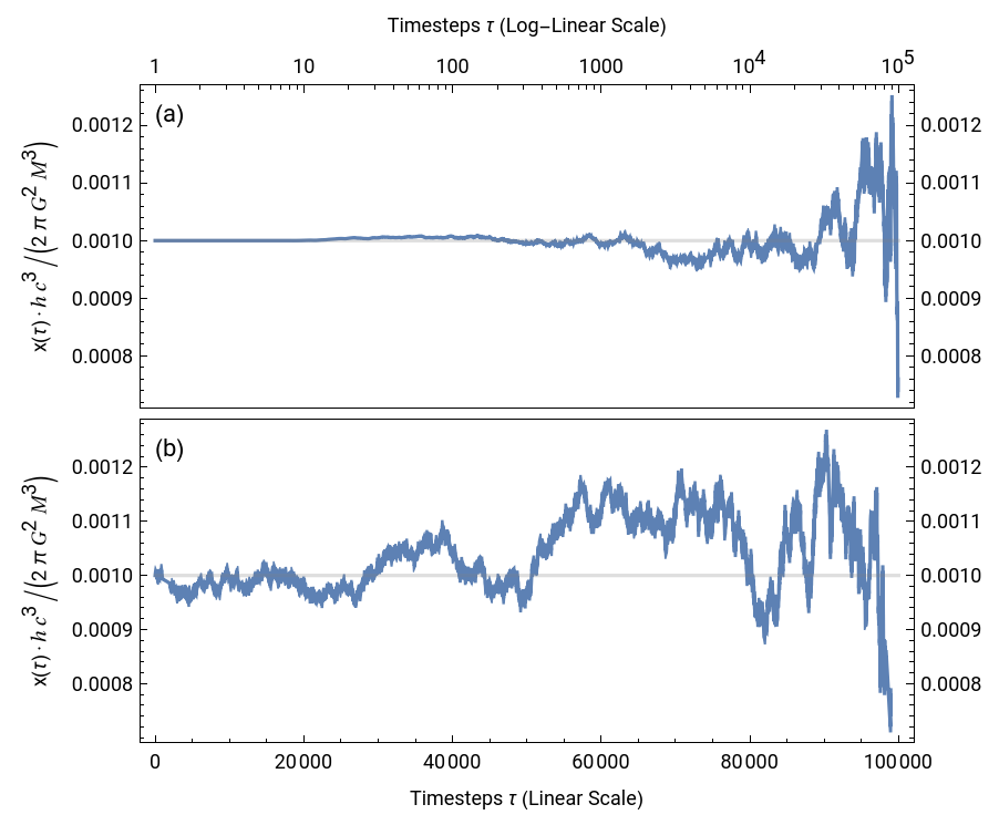
force[x_]:=(2EulerGamma/(3Pi))*(beta[t[x]]^(15)/(r[t[x]]p[t[x]]^(1/2))^3)(*Thequantadissipationforce,otherwiseobserver-timedependent*)forcedata=Table[force[i],{i,length}];(*Theproduceddatasetfromtheaboveforcefunction*)data=RandomVariate[NormalDistribution[0,1],length];kicks=Table[(data[[i]]/((r[t[i]])^3dt^(1/2))),{i,length}];(*Thestochasticnoisegenerator*)xo=10^(-3);x[1]=xo;(*Settingupaninitialcondition,veryclosetozero*)Do[dx=(forcedata[[i]]*a[i]+kicks[[i]])dt*xo/a[i];If[x[i]xo&&kicks[[i]]≤forcedata[[i]],dx=0];x[i+1]=x[i]+dx;If[x[i+1]<0,x[i+1]=0],{i,1,length}];tabel=Table[x[j],{j,length}];f=Interpolation[tabel];ResourceFunction["PlotGrid"]LogLinearPlot{f[i],xo},{i,1,length},Frame->True,PlotRangeAll,FrameLabel->{"x(τ)

·h

/(2π

)

",None},{None,"Timesteps τ (Log-Linear Scale)"},FrameTicks->{{All,All},{None,All}},FrameStyle->Directive[Black],PlotStyle->{{},{Gray,Opacity[0.25]}},Plot{f[i],xo},{i,1,length},Frame->True,PlotRangeAll,FrameLabel->{{"x(τ)

·h

/(2π

)

",None},{"Timesteps τ (Linear Scale)",None}},FrameTicks->{{All,All},{All,None}},FrameStyle->Directive[Black],PlotStyle->{{},{Gray,Opacity[0.25]}},Spacings->5,AspectRatio->0.85,PlotRange->All,PlotLabels->Column->Style["(a)",11,Black](*Producesa2-panelfigurefortheLog-linearscale(top)andthelinearscale(bottom)*)

Out[]=

Results

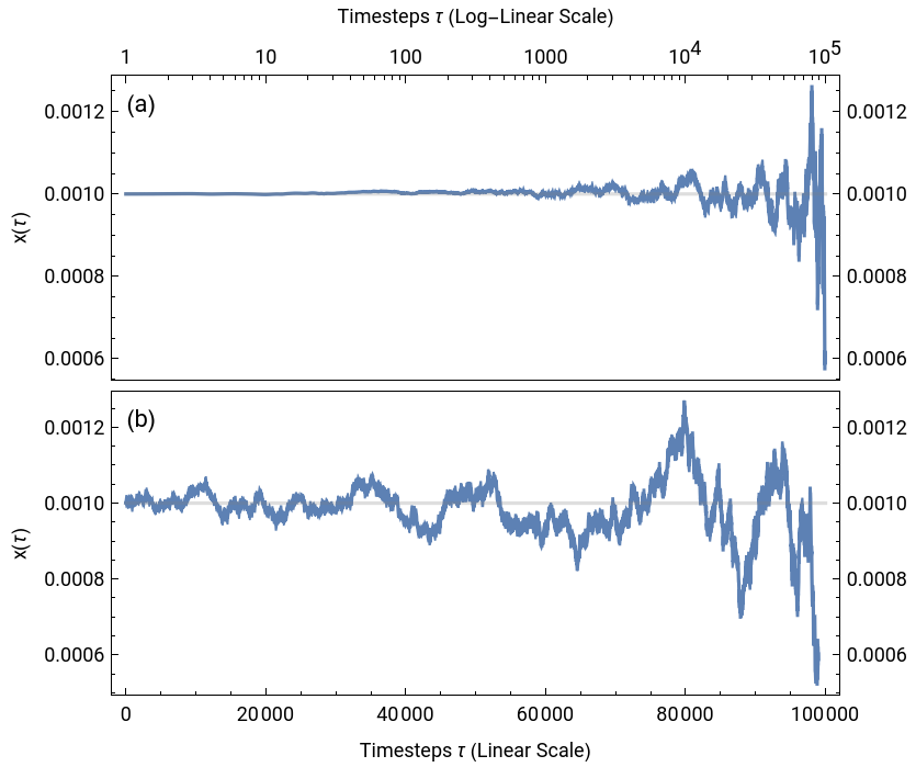
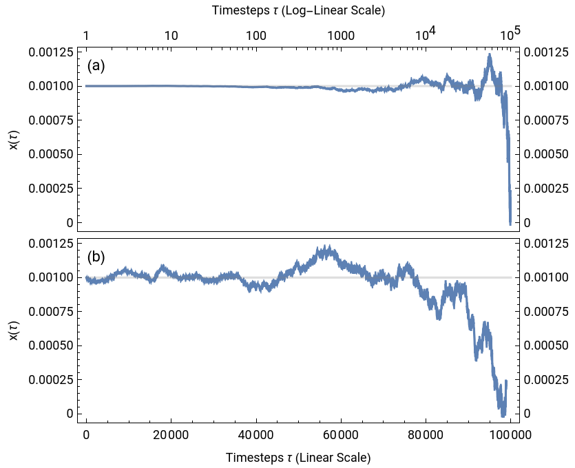
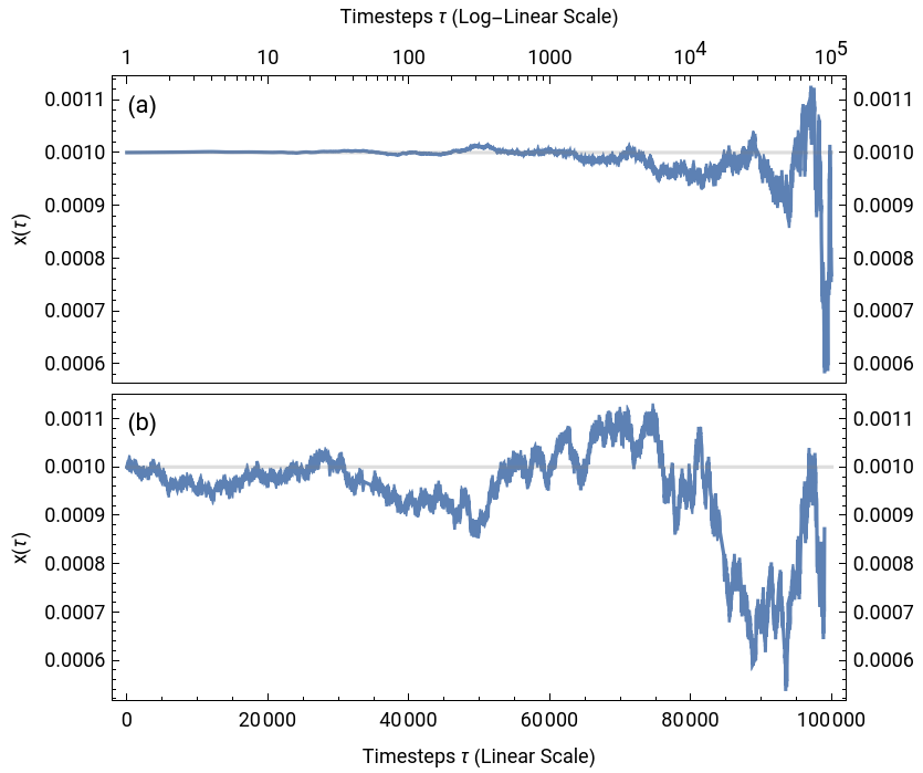
The results from the above code are never guaranteed to be replicated, providing a unique profile of the produced signal. However, the signals give a phenomenological translation of gravitational wave generation as graviton fluctuations. These can be seen in the provided sample figures:

◼

Current Article Figure

◼

Sample figures

◼

Old preprint figure

These generated signals (especially the log-linear scale) can be compared with actual gravitational wave signals (https://journals.aps.org/prl/abstract/10.1103/PhysRevLett.116.061102):

Signals under a Non-Gaussian Distribution

Even for gravitational wave detection, a Gaussian signal is a good approximation for extracting measurements. However, it is to be expected that non-Gaussianity (deviations from a pure Gaussian distribution) provides a realistic insight into these measurements. This can also be said for simulating graviton fluctuations. In the original article and the above code, the non-Gaussianity of graviton fluctuations comes from the imbalance between the “kicks” and the dissipation, showing that the kicks are more frequent than dissipation. If the gravitational field between the two inspiraling masses is resembled as a “graviton gas,” kicks from collisions with nearest neighbors happen more frequently than the dissipation of these gravitons as intermediate gravitational waves. If left under the normal distribution, non-Gaussianity comes from the kick-dissipation imbalance.

Another approach of non-Gaussianity is the alpha-stable distribution, where the stability factor α ∈ (1, 2] gauges the strength of “normality.” This hints at the application of off-equilibrium noise analysis to graviton fluctuations, but not to the stark degree of complex systems and self-organizing criticality. Thus, we can assume a near-Gaussian alpha-stable distribution with α=1.99. The above code can be revised for the near-Gaussian alpha-stable noise provided below:

Where the following results are produced:

◼

Current Article Figure

◼

Sample figures

◼

Old preprint figure

Notice the subtle difference in the later time-steps. Under the Gaussian noise, the lead-up to the spike is more sinusoidal. Here, the final spike appears pronounced after fluctuations around the initial position in some cases.

Discussion and Conclusion

This notebook is definitely detailed, but as a proof-of-concept, it is not meant to replace the more robust waveform models used in numerical relativity. Rather, it provides the graviton fluctuation description behind gravitational wave generation, and rather impressively, the graviton signals resemble quantitatively the macroscopic waveform profile of an excited sinusoidal “chirp” at later time-steps. And as a proof-of-concept, alternative descriptions of our measurable parameters are encouraged to be tested, to see if the resulting graviton fluctuations can better mimic gravitational wave signals. Pursuing the latter can only reinforce the quantum-classical correspondence between gravitons and gravitational waves.

CITE THIS NOTEBOOK

Gravitational wave generation via the Einstein-Langevin equation
by Noah MacKay
Wolfram Community, STAFF PICKS, April 7, 2025
https://community.wolfram.com/groups/-/m/t/3440876