Computation of the Bifurcation Diagram
for the Three-Variable Autocatalator
Authors: Housam Binous and Ahmed Bellagi
Computation of the Bifurcation Diagram
for the Three-Variable Autocatalator
Authors: Housam Binous and Ahmed Bellagi
for the Three-Variable Autocatalator
Authors: Housam Binous and Ahmed Bellagi
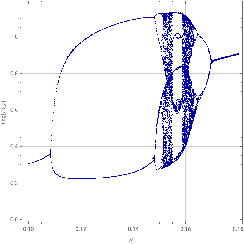
Consider a chemical reaction such as the shift conversion: . To study its chemical kinetics, it is written in abstract form as . The rate of this reaction is given by , where is the rate constant and , , and are the concentrations of the species , , and .Hypothetically, the autocatalator's steps are the following:Here is a precursor with constant concentration, is the final product, , , and are intermediate chemical species, , , , , , and are rate constants for the individual reactions, and , , , , and are the concentrations of the hypothetical chemical species , , , , and . This hypothetical reaction scheme is a model for a three-variable autocatalator. The autocatalytic reaction occurs in the step , with catalyzing its own formation. This step introduces the nonlinear term a in the governing equations, necessary in order to obtain sufficient complexity for chaos to occur. The rate equations for the three intermediate species can be written in the form:=+c-a-a,=a+a-b,=b-c.The corresponding dimensionless rate equations are:=κ+μγ-α-α,,,where , , and are the dimensionless concentrations of , , and , and the four parameters , , , and depend on the rates of the individual reactions and the concentration of the precursor.We compute the bifurcation diagram for this nonlinear chemical system. This bifurcation diagram, a remerging Feigenbaum tree, was first given in Ref. 1.References:[1] B. Peng, S. K. Scott, and K. Showalter, "Period Doubling and Chaos in a Three-Variable Autocatalator," The Journal of Physical Chemistry, 94(13), 1990 pp. 5243–5246.[2] S. Lynch, Dynamical Systems with Applications using Mathematica, Boston: Birkhäuser, 2007.
CO+O+
H
2
CO
2
H
2
X+Y→W+Z
r==kxy
dz
dt
k
x
y
z
X
Y
Z
reactionrateP→AP+C→A+CcA→BaA+2B→3BaB→CbC→Dc
k
0
p
0
k
c
p
0
k
u
k
1
2
b
k
2
k
3
P
D
A
B
C
k
0
k
c
k
u
k
1
k
2
k
3
p
0
d
a
b
c
P
D
A
B
C
A+2B→3B
B
k
1
2
b
da
dt
k
0
p
0
k
c
p
0
k
u
k
1
2
b
db
dt
k
u
k
1
2
b
k
2
dc
dt
k
2
k
3
dα
dτ
2
β
σ=α+α-β
dβ
dτ
2
β
δ=β-γ
dγ
dτ
α
β
γ
A
B
C
κ
μ
δ
σ
Bifurcation Diagram - Computation takes over one hour.
In[]:=
sol[μ_]:=NDSolve[{D[α[t],{t,1}]κ+μγ[t]-α[t]β[t]^2-α[t],σD[β[t],{t,1}]α[t]β[t]^2+α[t]-β[t],δD[γ[t],{t,1}]β[t]-γ[t],α[0]1,β[0]1,γ[0]1},{α[t],β[t],γ[t]},{t,0,20}]
In[]:=
κ=10;δ=210^-2;σ=510^-3;
In[]:=
iterate=Compile[{μ},{f=sol[μ];Map[{μ,#}&,FindMinValue[Log[10,γ[t]/.f],{t,#,#+0.01}]&/@Table[i,{i,4,10.0,0.01}]]}]
Out[]=
CompiledFunction


In[]:=
LaunchKernels[]
Out[]=
KernelObject,KernelObject,KernelObject,KernelObject
In[]:=
pts=Parallelize[Table[iterate[μ],{μ,0.10,0.18,0.0001}]];
In[]:=
ListPlot[Flatten[pts,1],PlotStyleTable[{PointSize[0.003],Darker@Blue},{i,1,Length[pts]}],FrameTrue,FrameLabel{Style["μ",Italic],Style["Log[10,γ]",Italic]},ImageSize{400,400},AspectRatio1,GridLines->Automatic]
Out[]=