Bold Predictions with the Logistic Epidemic Model
Bold Predictions with the Logistic Epidemic Model
This notebook can be used to track the coronavirus in the United States, looking at each state individually. A logistic growth model has been successful in predicting the course of epidemics in China and South Korea. A detailed mathematical description of the logistic model has been posted. The data source is the Wolfram Data Repository for the epidemic. Three graphics, which are described below, are used to describe the status of the epidemic in each state. This notebook can be downloaded to follow the epidemic and see how the model performs.
Procedures
Procedures
In[]:=
stateEntityList=Uncompress["1:eJylmN9u2jAUxqv9abeV7WKadp09w56ggrakNElFKKy7M4khFsGubANlTz8ndkJCJ+WMI1XUIOv3+djnHH/Jj7kYL36enZ2pd+bjnim9eNv8Fl+YwVVO5mRN4jfF+H5R/FPn5uOaa6b38ffi53TNuJkviWZbOmBbppjgduo/WT0zfuRM0zTWRFN1JHtup6qVUx2drtpAdYiW65Psj+BO9TcyVsfqkP1QTl0RroiyuuPTdVuwDuFPZtAnOVsIyZkNuX91uvQRDhB1X+RCklRY6QgXdQ3rEL4s53JOE82Sjbbak9O1j3mAuAc0Jzsiaak9uMbFXcMA2X1jtoil9qhvkJVcsQCyt1TIpcuwW0SGNVmABjI0+8JYqTr0cQ3EoTpE35uBn5LMJrQ/OF3zQAKkk5/njAtmm4ePONYWDHCuPk8Zcc3SD3HnWrE6ZIuBL3ZOE5FLNQiQSKNDbx7FuEQagTpzcRAjyvUmWe2t7BPuVGtYh/DHYiA2BlOd6z1ij9s0QPEEhHHbFQNEVzyQANscELnPCU+tKqJkW7AO4c/lXKVIkm0U1drmVoDY6tdESOwsydiScKuOaJEtGCDFAmbuSyW0TbEA0TraNMDVHzClir/nZ3szBIiCPuaBtlwpsZFOG2l5ahigVweC66qmA4TdabIA8YZ0LmsbHyKtTg0D9OyQbolzOuEU17MdClDTId15Q7J+Vhlz7i4cnq7ds8QDEODnixXcUamovTfCO1xpGZyjAbUD+sIS63/CAK3taKA823lPQq6sMuK2vLCwktWh+6WYKqTOvD6Rwtgml259XBsvkTWxYw29eg0Dsqoaaoi4xi4roOMB/FiUMXviESLZaxDgsKNVbqyxeyMRId4NtGCAphJJuhT2uowQD+kNFOB4Hyjnap9vSfWQ/oDwCa+AgAWMM5FSz1e1TRojrMJlBXQ8QI3FYnNcYzGyxkrk/9SYXUOjxmJkjZVAWI0VzXBCC4+jqL1VJkjHdKABTPmEvriHn8kvnCm3JEBHedQkKxUfEU6lBgHc0ZTKtTE1peYU6Y4qFqCRTZlcsqqsp4iybsEAV/WMGEfBl9o1sxnytV8DB3BJM6q01wp9hnBoPUeEhl/k/4ypRHDFXPSIdtamATJtthcGu7TCSJ9SsTpkv5nBoOCxRHti4fVFvlnP3dYPEJ30awMcLWrs8XL+AsiaSC0="];
In[]:=
epidemicDates[NLM_FittedModel]:=DatePlus{2020,1,21},Floort0-/.NLM@"BestFitParameters",DatePlus{2020,1,21},Ceilingt0+/.NLM@"BestFitParameters";Clear[differenceLogReport];differenceLogReport[cases0_List,opts___]:=Module{nlm,cases,dates,ygrid},If[Head[cases0[[1]][[1]]]===DateObject,cases=Transpose[{DateDifference[{2020,1,21},#][[1]]&/@cases0[[All,1]],cases0[[All,2]]}],If[Head[cases0[[1]][[1]]]===Integer,cases=cases0,Return[]]];nlm=NonlinearModelFitcases,,{{k,0.3},{L,cases[[-1]][[2]]},{t0,cases[[-1]][[1]]}},t;Print[nlm@"BestFitParameters"];dates=epidemicDates[nlm];dtlist=DateRange[DatePlus[{2020,1,21},cases[[2]][[1]]],dates[[2]]];ygrid=Join[Range[0,20]/10.,{{k/.nlm@"BestFitParameters",{Dashed,Thick}}}];Print@DateListPlot[{Tooltip[#,#]&/@Transpose[{dtlist,Differences@Log[nlm[#]&/@Range[cases[[1]][[1]],DateDifference[{2020,1,21},dates[[2]]][[1]]]]}],Tooltip[#,#]&/@Transpose[{Take[dtlist,Length@cases-1],Differences@Log@N@cases[[All,2]]}]},opts,JoinedFalse,FrameTrue,FrameLabel{None,"Daily Growth Rate"},PlotLegends{"Predicted","Actual"},GridLines{Automatic,ygrid}];{nlm,TimeSeries[cases],dates};
Log[-1+L]
k
Log[-1+L]
k
L
1+
-k(t-t0)
In[]:=
Clear[modelLogFitDLP];modelLogFitDLP[NLM_,data_,opts___]:=Module{p0,p1,dates},dates=epidemicDates[NLM];p0=LogPlotNLM,{t,AbsoluteTime[DatePlus[{2020,1,21},data[[1]][[1]]]],AbsoluteTime[dates[[-1]]]},GridLinesAutomatic,PlotLegends{"Fit"};p1=DateListLogPlot[data[[All,2]],{DatePlus[{2020,1,21},data[[1]][[1]]],DatePlus[{2020,1,21},data[[-1]][[1]]]},opts,JoinedFalse,PlotStyleRGBColor[0.880722,0.611041,0.142051],FrameTrue,FrameLabel{None,"Cases"},GridLinesAutomatic];Show[p1,p0,PlotRangeAll];
t-AbsoluteTime[{2020,1,21}]
86400
In[]:=
Clear[usReport];usReport[stateID_String]:=Module[{state,ds,ts,res},state=Select[stateEntityList,#[[2]]stateID||#[[1]]stateID&][[1]][[3]];ds=covid19Data@Select[#"AdministrativeDivision"===state&];ts=Select[Normal@ds[All,"ConfirmedCases"][[1]],#[[2]]>12&];Print@DateListLogPlot[Tooltip[#,#]&/@ts,JoinedFalse,PlotStyleRGBColor[0.880722,0.611041,0.142051],FrameTrue,FrameLabel{None,"Cases"},GridLinesAutomatic,PlotLabelCommonName@state];res=differenceLogReport[ts,PlotLabel"Daily Log Case Differences"];Print@modelLogFitDLP[res[[1]],Normal@res[[2]],PlotLabel"Logistic Model Fit"];Print["Epidemic Duration ",res[[3]],DateDifference[Sequence@@res[[3]]]];res];
In[]:=
ro=ResourceObject["Epidemic Data for Novel Coronavirus COVID-19"];
In[]:=
(*DeleteObject[ro]*)(*MaybeneededifResourceObjectdoesnotupdateonlocalcomputer*)
In[]:=
covid19Data=ResourceData["Epidemic Data for Novel Coronavirus COVID-19"];
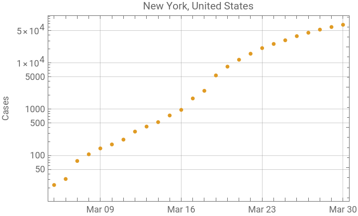
Currently New York is the epicenter of the epidemic in the U.S. but it is beginning to show signs that quarantine measures are working.
In[]:=
nyRes=usReport["NY"];
{k0.338632,L87499.2,t065.7294}



Epidemic Duration {{2020,2,22},{2020,4,30}}
In[]:=
njRes=usReport["NJ"];
{k0.359745,L30815.2,t068.6113}
Graphic Description
Graphic Description
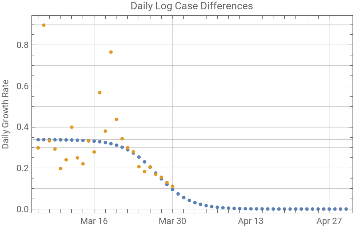
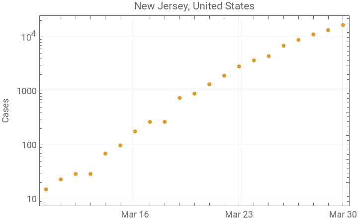
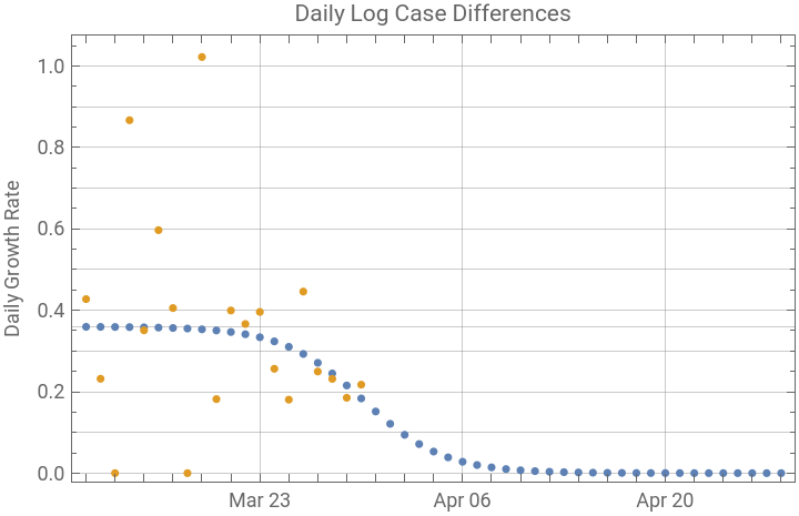
The report is generated by entering the state name or postal code into usReport[...] as a string. The first graph is a logarithmic plot of the cumulative number of cases by day. A lot of information about the state of the epidemic can be gleaned by looking at the plot carefully. Exponential growth on a log plot will be linear. Any section of the plot where there is a concave upward trend would indicate numbers growing faster than exponentially. This can happen when information accumulates more rapidly or perhaps when more testing is happening, but it is not a feature expected for virus spread, which should be linear on the log plot until there is effective quarantine. Generally a reasonable logistic fit to the data will not happen until the later points on the log plot show some downward concavity, indicating that a quarantine process is slowing the rate of spread of the viral infection.
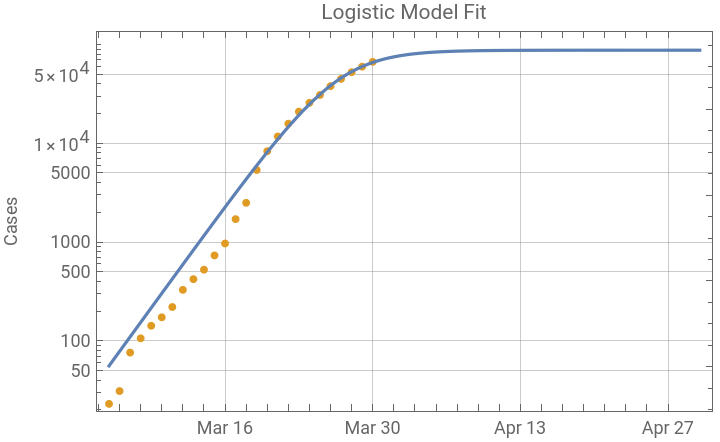
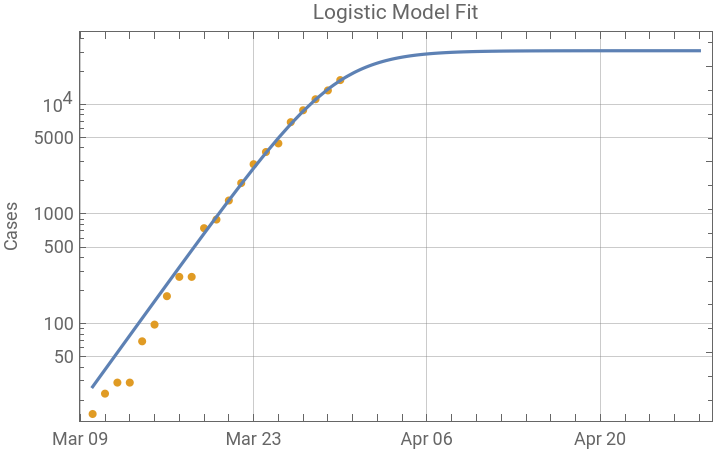
The third graphic is a log plot of the logistic model fit and the data points; it has the same data points in orange as the first graph, but extends the predicted curve to the end of the epidemic. The points show an interesting pattern which is not apparent on a linear plot. The early points do not have much effect in determining the fit. The default method is used in NonlinearModelFit, and this is allowing the large magnitude of later data points to dominate the smaller residual differences in the early points. This is actually helpful for the analysis, because the early data is collected before much is known about the contacts of infected individuals, and more severely ill people are easier to count early in the epidemic, when there was not adequate testing available. As the cumulative case numbers become larger, small counting errors will have much less effect in the data collection and reporting, which will always lag the state of the epidemic because there is an incubation period before the infection becomes apparent.
The function also outputs a result:
The first component is the NonlinearModelFit which can be used to get all the information about the fit. The fit parameters are shown below. k is the growth rate of the underlying exponential process. L is the predicted maximum case number and t0 is the estimated time of the peak of the epidemic on an arbitrary time scale in days, where day zero is {2020, 1, 21}. The predicted peak is calculated below.
Some other uses of the results are shown below. A parameter confidence interval table is shown and a plot of the function and first and second derivatives is below.
The second element is the time series in the form used to calculate the NonlinearModelFit.
The third element is the predicted dates of the beginning and end of the epidemic, calculated for times when the case count is 1 and L - 1.