ABSTRACT (original article): Numerous tabletop experiments have been dedicated to exploring the manifestations of screened scalar field dark energy, such as symmetron or chameleon fields. Precise theoretical predictions require simulating field configurations within the respective experiments. This paper focuses onto the less-explored environment-dependent dilaton field, which emerges in the strong coupling limit of string theory. Due to its exponential self-coupling, this field can exhibit significantly steeper slopes compared to symmetron and chameleon fields, and the equations of motion can be challenging to solve with standard machine precision. We present the first exact solution for the geometry of a vacuum region between two infinitely extended parallel plates. This solution serves as a benchmark for testing the accuracy of numerical solvers. By reparametrizing the model and transforming the equations of motion, we show how to make the model computable across the entire experimentally accessible parameter space. To simulate the dilaton field in one- and two-mirror geometries, as well as spherical configurations, we introduce a non-uniform finite difference method. Additionally, we provide an algorithm for solving the stationary Schrödinger equation for a fermion in one dimension in the presence of a dilaton field. The algorithms developed here are not limited to the dilaton field, but can be applied to similar scalar-tensor theories as well. We demonstrate such applications at hand of the chameleon and symmetron field. Our computational tools have practical applications in a variety of experimental contexts, including gravity resonance spectroscopy (qBounce), Lunar Laser Ranging (LLR), and the upcoming Casimir and Non-Newtonian Force Experiment (cannex). A Mathematica implementation of all algorithms is provided. CITATION (original article): Hauke Fischer and René I.P. Sedmik, Numerical methods for scalar field dark energy in tabletop experiments and Lunar Laser Ranging, JCAP10(2024)026. https://doi.org/10.1088/1475-7516/2024/10/026
Introduction
Introduction
This notebook contains more explanation on the usage of the code https://zenodo.org/records/10491446 that contains
the algorithms developed in the paper “Numerical Methods for Scalar Field Dark Energy in Tabletop Experiments and Lunar Laser Ranging”.
the algorithms developed in the paper “Numerical Methods for Scalar Field Dark Energy in Tabletop Experiments and Lunar Laser Ranging”.
The notebook is structured as follows:
◼
Section 1 shows how to simulate the two mirror solution as shown in Figs. 4-6 in the paper. This specific geometry is used to model the CANNEX experiment, as elaborated on in the paper.
◼
Section 2 provides the code to generate the simulations shown in Fig. 7, which is used to simulate spherical geometries as needed for Lunar Laser Ranging (LLR).
◼
Section 3 provides the code to generate the one mirror solution as well as the solution of the Schrödinger equation shown in Fig. 8. This can be used to model the qBounce Experiment, as elaborated on in the paper.
In the notebook, the dilaton field parameter γ in the paper is denoted as β.
Section 1: CANNEX (Figs. 4-6)
Section 1: CANNEX (Figs. 4-6)
Section 1.1 has to be activated first, to define all experimental parameters relvant to CANNEX.
Section 1.2 defines the necessary functions to solve the non-linear system of equations given by (5.9) for a two mirror geometry in the paper, and elaborated on in the appendix.
Section 1.3 Is used to define the non-uniform FDM mesh, as elaborated on in Section 5.2 in the paper. The parameters are set such at the moment that by just activating the cell, the mesh is suitable to simulate all fields in Section 1.
Section 1.4-1.7 show how to use the code to reproduce the examples given in the paper. In order to run these sections, section 1.1-1.3 need to be activated first.
Section 1.1: Define parameters
Section 1.1: Define parameters
Section 1.2: Define functions
Section 1.2: Define functions
Section 1.3: Define mesh, plate separation etc.
Section 1.3: Define mesh, plate separation etc.
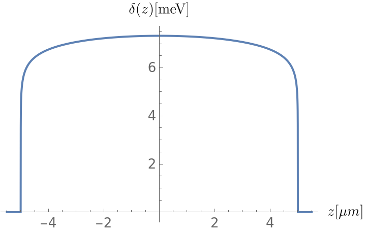
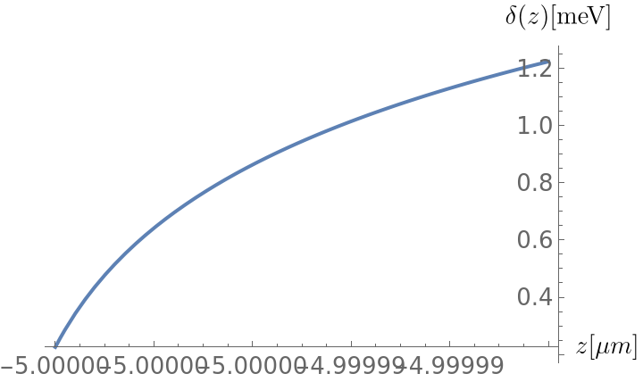
Section 1.4: Dilaton field Figure 4
Section 1.4: Dilaton field Figure 4
Up: the dilaton field is shown from −5.5 µm to 5.5 µm. Down: the field is shown from −5 µm to (−5 + 10−5) µm to illustrate the extreme slopes near the transition into the vacuum region.
In[]:=
Clear[ϕρ,Veff,DVeff,DDVeff]ϕM[A_,λ_,β_,ρ_]:=SetPrecision[mpl/λIf[2*Log10[λ]+β-Log10[A]-Log10[ρ]<1000000,ProductLog[(λ^210^β)/(Aρ)],Log[λ^2/(Aρ)]+1/(6(βLog[10]+Log[λ^2/(Aρ)])^3)(6βLog[10](βLog[10]+Log[λ^2/(Aρ)])^3-6(-1+βLog[10]+Log[λ^2/(Aρ)])(1+β^2Log[10]^2+2βLog[10]Log[λ^2/(Aρ)]+Log[λ^2/(Aρ)]^2)Log[βLog[10]+Log[λ^2/(Aρ)]]+3(-3+βLog[10]+Log[λ^2/(Aρ)])Log[βLog[10]+Log[λ^2/(Aρ)]]^2+2Log[βLog[10]+Log[λ^2/(Aρ)]]^3)],50]ϕρ[A_,λ_,β_,ρ_]:=SetPrecision[0,16]BETA[A_,λ_,β_,ϕ_]:=SetPrecisionA*,16DVeff[ϕ_,A_,λ_,β_,ρ_]:=SetPrecision-*ρM*Exp[-λ*ϕ/mpl]+*ρ,16DDVeff[ϕ_,A_,λ_,β_,ρ_]:=SetPrecision*ρM*Exp[-λ*ϕ/mpl]+,16
ϕ
mpl
BETA[A,λ,β,ϕM[A,λ,β,ρM]]
mpl
BETA[A,λ,β,ϕM[A,λ,β,ρM]+ϕ]
mpl
λ*BETA[A,λ,β,ϕM[A,λ,β,ρM]]
2
mpl
A*ρ
2
mpl
In[]:=
Clear[CPrec,FINAL,A2,β,λ,SEED,Guess2]CPrec=15;(*Theinternalprecissionusedis5xCPrec*)λ=SetPrecision[10^(31),1000];A2=10^45;β=10^0;Clear[ρV,rhoV]ρV=0;rhoV=ρV;Seed={};For[i=1,i<=Length[points],i++,AppendTo[Seed,Block[{$MaxExtraPrecision=1000},0]]]Prec=100;MAX=100;Timing[{Vectorform,SOLUTION2}=SOLVEFD[A2,λ,β,points,Prec,MAX,Seed,DVeff,DDVeff];]MIN=50;COMP1=Plot{(SOLUTION2[z*])*},{z,-1.1*5,1.1*5},PlotRange->Full,FrameLabel->{Style["x-axis",Bold,12],Style["y-axis",Bold,12]},LabelStyle->{FontFamily->"Arial",FontSize->13},AxesLabel->{MaTeX["z[\\mu m]",Magnification->1.2],MaTeX["\\delta (z)[\\text{meV}]",Magnification->1.2]},PlotStyle->{Thick},Exclusions->Noneδ=SetPrecision[1*,1000];COMP2=Plot{SOLUTION2[z*]*},{z,-5,-5+δ},PlotRange->Full,FrameLabel->{Style["x-axis",Bold,12],Style["y-axis",Bold,12]},LabelStyle->{FontFamily->"Arial",FontSize->13},AxesLabel->{MaTeX["z[\\mu m]",Magnification->1.2],MaTeX["\\delta (z)[\\text{meV}]",Magnification->1.2]},PlotStyle->{Thick},Exclusions->None
-6
10
9
10
-5
10
-6
10
9
10
Out[]=
{25.9063,Null}
Out[]=
Out[]=
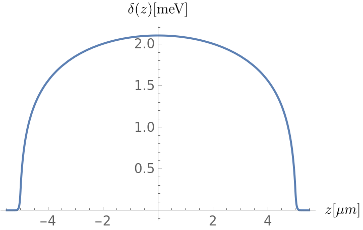
Section 1.5: Dilaton field Figure 5
Section 1.5: Dilaton field Figure 5
In[]:=
Clear[CPrec,FINAL,A2,β,λ,SEED,Guess2]CPrec=15;(*Theinternalprecissionusedis5xCPrec*)λ=SetPrecision[10^(31),1000];A2=10^13;β=10^24;Clear[ρV,rhoV]ρV=0;rhoV=ρV;Seed={};For[i=1,i<=Length[points],i++,AppendTo[Seed,Block[{$MaxExtraPrecision=1000},0]]]Prec=15;MAX=100;Timing[{Vectorform,SOLUTION2}=SOLVEFD[A2,λ,β,points,Prec,MAX,Seed,DVeff,DDVeff];]Plot{(SOLUTION2[z*])*},{z,-1.1*5,1.1*5},PlotRange->Full,FrameLabel->{Style["x-axis",Bold,12],Style["y-axis",Bold,12]},LabelStyle->{FontFamily->"Arial",FontSize->13},AxesLabel->{MaTeX["z[\\mu m]",Magnification->1.2],MaTeX["\\delta (z)[\\text{meV}]",Magnification->1.2]},PlotStyle->{Thick},Exclusions->None,WorkingPrecision->100
-6
10
9
10
Out[]=
{10.7344,Null}
Out[]=
Section 1.6: Chameleon field Figure 6
Section 1.6: Chameleon field Figure 6
Section 2: LLR (Fig. 7)
Section 2: LLR (Fig. 7)
Section 2.1 has to be activated first, to define all experimental parameters relevant to LLR.
Section 2.2 defines the necessary functions to solve the non-linear system of equations given by (5.9) in the paper for a spherical geometry, and elaborated on in the appendix.
Section 2.3 Is used to define the non-uniform FDM mesh, as elaborated on in Section 5.2 in the paper. The parameters are set such at the moment that by just activating the cell, the mesh is suitable to simulate the field in Section 2.4.
Section 2.4 shows how to use the code to reproduce the example given in the paper. In order to run these sections, section 2.1-2.3 need to be activated first.
Section 2.3: Define mesh, plate separation etc.
Section 2.3: Define mesh, plate separation etc.
Section 3: qBounce (Fig. 8)
Section 3: qBounce (Fig. 8)
Section 3.1 has to be activated first, to define all experimental parameters relevant to qBounce.
Section 3.2 defines the necessary functions to solve the non-linear system of equations given by (5.9) in the paper for a one mirror geometry, and elaborated on in the appendix, as well as for solving the Schrödinger equation as explained in Section 6 in the paper.
Section 3.3 Is used to define the non-uniform FDM mesh, as elaborated on in Section 5.2 in the paper. The parameters are set such at the moment that by just activating the cell, the mesh is suitable to simulate the field in Section 3.4.
Section 3.4 shows how to use the code to reproduce the example given in the paper. In order to run these sections, section 3.1-3.3 need to be activated first.
Section 3.4: Solution Schrödinger equation Figure 8
Section 3.4: Solution Schrödinger equation Figure 8
I start by defining a complete mesh and the potential
CITE THIS NOTEBOOK
CITE THIS NOTEBOOK
Numerical methods for scalar field dark energy in tabletop experiments and Lunar Laser Ranging
by Hauke Fischer & René I.P. Sedmik
Wolfram Community, STAFF PICKS, December 4, 2024
https://community.wolfram.com/groups/-/m/t/3333622
by Hauke Fischer & René I.P. Sedmik
Wolfram Community, STAFF PICKS, December 4, 2024
https://community.wolfram.com/groups/-/m/t/3333622