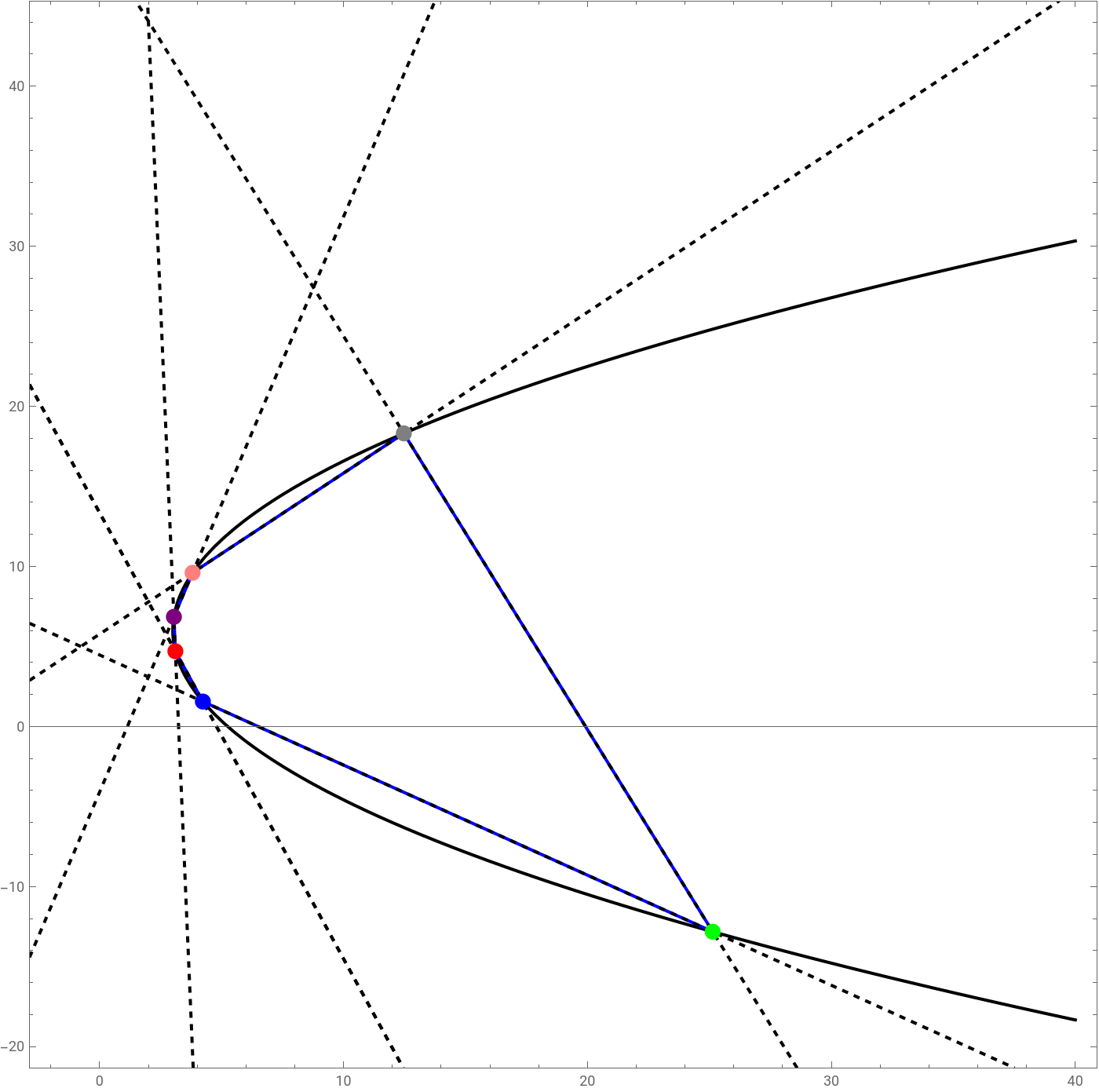
PascalTheorem::usage=" In any hexagon inscribed in a conical section, the continuations of opposite sides meet on a straight line, called the Pascal line. This property is repeated in Geometry, there is also the Monge's theorem and the Desargues' theorem. References: Personal, based in the Pascal's theorem. ";
Development:
Obtaining the vertices of the hexagon in numerical form:
In[]:=
r=2;k=4;d=-2;n=6;ρ=;x1=4;y1=6;k1=;TablePoint{4-d,y1}++-{(r+ρ)Cos[t1+2πk1]+x1-(4-d),(r+ρ)Sin[t1+2πk1]+y1-6},t1,0,2π,//FullSimplify
2Sin
π
n
1-Sin
π
n
3
5
2
k
2
((r+ρ)Cos[t1+2πk1]+x1-(4-d))
2
((r+ρ)Sin[t1+2πk1]+y1-6)
2
ρ
2π
n
Point4-,6-4,6+,Point2+,6-4Cot,Point24+,2+,Point2+,6+4Tan,Point4-,6-4
2
5
1-
,Point2-2
5
2
-1+Sin
π
30
4Cos
π
30
-1+Sin
π
30
2
Csc
π
15
π
15
5
,6+45+2
,Point2+5
2
1+Sin
π
30
8
1+Tan
π
60
2
Sec
π
15
π
15
2
5
1-
;2
5
In[]:=
Showr=2;k=4;d=-2;n=6;ρ=;x1=4;y1=6;k1=;ContourPlot[-16x-12y+84==0,{x,0,40},{y,-20,40},ContourStyle->{Black,Thick},PlotPoints->50],TableGraphicsBlue,Thick,Line{4-d,y1}++-{(r+ρ)Cos[t1+2πk1]+x1-(4-d),(r+ρ)Sin[t1+2πk1]+y1-6},{4-d,y1}++-(r+ρ)Cost1++2πk1+x1-(4-d),(r+ρ)Sint1++2πk1+y1-6,t1,0.00001,2π,,TableGraphicsBlack,Thick,Dashed,InfiniteLine{4-d,y1}++-{(r+ρ)Cos[t1+2πk1]+x1-(4-d),(r+ρ)Sin[t1+2πk1]+y1-6},{4-d,y1}++-(r+ρ)Cost1++2πk1+x1-(4-d),(r+ρ)Sint1++2πk1+y1-6,t1,0,2π,,GraphicsRed,PointSize[0.015],Point4-,6-4,6+,GraphicsGreen,PointSize[0.015],Point2+,6-4Cot,GraphicsGray,PointSize[0.015],Point24+,2+,GraphicsPurple,PointSize[0.015],Point2+,6+4Tan,AxesTrue,BoxRatiosAutomatic,AxesOrigin{0,0},ImageSize700,PlotRange{{-2,40},{-20,44}}
2Sin
π
n
1-Sin
π
n
3
5
2
y
2
k
2
((r+ρ)Cos[t1+2πk1]+x1-(4-d))
2
((r+ρ)Sin[t1+2πk1]+y1-6)
2
ρ
2
k
2
(r+ρ)Cost1++2πk1+x1-(4-d)
2π
n
2
(r+ρ)Sint1++2πk1+y1-6
2π
n
2
ρ
2π
n
2π
n
2π
n
2
k
2
((r+ρ)Cos[t1+2πk1]+x1-(4-d))
2
((r+ρ)Sin[t1+2πk1]+y1-6)
2
ρ
2
k
2
(r+ρ)Cost1++2πk1+x1-(4-d)
2π
n
2
(r+ρ)Sint1++2πk1+y1-6
2π
n
2
ρ
2π
n
2π
n
2π
n
2
5
1-
,GraphicsBlue,PointSize[0.015],Point2-2
5
2
-1+Sin
π
30
4Cos
π
30
-1+Sin
π
30
2
Csc
π
15
π
15
5
,6+45+2
,GraphicsPink,PointSize[0.015],Point2+5
2
1+Sin
π
30
8
1+Tan
π
60
2
Sec
π
15
π
15
Out[]=
Obtaining the equations of the opposite sides:
GreenBlue line and PinkPurple, form the point 1:
In[]:=
Solvey-6-4Cot2--2+==6+-6-4Cotx-2+,y-2+2+-2+==6+4Tan-2+x-2+,{x,y}//FullSimplify
π
15
2
-1+Sin
π
30
2
Csc
π
15
4Cos
π
30
-1+Sin
π
30
π
15
2
Csc
π
15
8
1+Tan
π
60
2
Sec
π
15
2
1+Sin
π
30
π
15
8
1+Tan
π
60
2
1+Sin
π
30
x2,y2+;
8
1+Cot
π
20
BlueRed line and GrayPink, form the point 2:
In[]:=
Solvey-6+4--2-==6-4x-2-,y-6+4-24+-6+4
4Cos
π
30
-1+Sin
π
30
2
5
2
-1+Sin
π
30
1-
-6+2
5
4Cos
π
30
-1+Sin
π
30
2
-1+Sin
π
30
5+2
2+5
2
1+Sin
π
30
5
==2+8
1+Tan
π
60
5+2
x-24+5
5
,{x,y}//FullSimplifyx2,y6+4;

RedPurple line and GreenGray, form the point 3:
In[]:=
Solvey-6-4-4-==6+4Tan-6-4,y-6-4Cot24+==6+4x-2+,{x,y}//FullSimplify
1-
2+2
5
2
Sec
π
15
2
5
π
15
1-
x-4-2
5
2
5
π
15
5
-2+2
Csc
π
15
5+2
-6-4Cot5
π
15
2
Csc
π
15
x2,y4Cos3+2-15-6+5+3-2Sin++3Sin+10-25+2;
π
15
55-2
+155
5+2
+210-35
55+2
Cos5
2π
15
5
+255+2
Sin5
2π
15
5
2+3Cos7π
30
7π
30
105+
-3+2Cos5
7π
30
7π
30
165-30
+15+6
5
55+2
Cos5
π
15
5-2
5
2
Sin
π
30
5
Sinπ
15
Complete graph:
The graph shows Pascal’s line.