In[]:=
SpaceCurve2::usage="Parametric equations are indicated below. References: Hollis, Selwyn. CalcLabs with Mathematica, Multivariable Calculus. 4a Ed., Cengage Learning: p.46, 2010; Personal ";f[x_,y_]:=4--;g[x_,y_]:=+2-xy;Show[surf1=Plot3D[f[x,y],{x,-3,3},{y,-3,3},ColorFunction"BlueGreenYellow",MeshFalse],surf2=Plot3D[g[x,y],{x,-3,3},{y,-3,3},ColorFunction"LightTemperatureMap",MeshFalse],AxesLabel->(Style[#,15,Blue]&/@{"X","Y","Z"}),AxesOrigin{0,0,0},AxesTrue,BoxedFalse,BoxRatiosAutomatic]f[rCos[t],rSin[t]]==g[rCos[t],rSin[t]];roft=r/.First@Solve[%,r]//Simplify;z[t_]:=g[roftCos[t],roftSin[t]];γ[t_]:={roftCos[t],roftSin[t],z[t]};
2
x
2
y
2
x
2
y
Out[]=

In[]:=
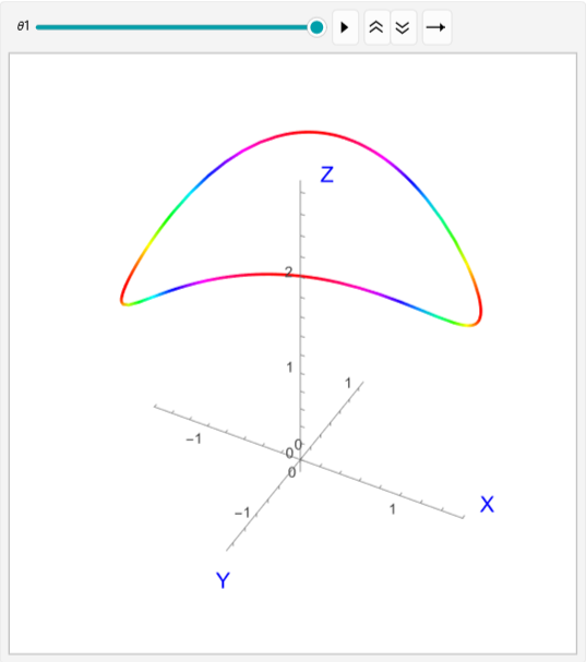
Animateγ[t_]:=-,-,-+;ParametricPlot3D[γ[t],{t,0,θ1},AxesLabel->(Style[#,15,Blue]&/@{"X","Y","Z"}),AxesOrigin{0,0,0},MeshFalse,AxesTrue,ColorFunctionFunction[{x,y,z},Hue[z]],BoxedFalse,PlotRangeAll,PerformanceGoal"Quality"],{θ1,0.1,2π,0.1},AnimationRunningFalse
2Cos[t]
2-Cos[t]Sin[t]+3
2
Cos[t]
2
Sin[t]
2Sin[t]
2-Cos[t]Sin[t]+3
2
Cos[t]
2
Sin[t]
4
2
Cos[t]
2-Cos[t]Sin[t]+3
2
Cos[t]
2
Sin[t]
4Cos[t]Sin[t]
2-Cos[t]Sin[t]+3
2
Cos[t]
2
Sin[t]
8
2
Sin[t]
2-Cos[t]Sin[t]+3
2
Cos[t]
2
Sin[t]
Out[]=