Simulating a Multiple Server Queue
Simulating a Multiple Server Queue


In queuing theory, the simplest model is called the M/M/1 or M/M/c model (Markovian arrivals, Markovian service, and 1 or servers). Customers arrive at a facility and either get served immediately by a free server or join a queue that waits for a server to become available. Standard notation is:
c
λ
1/λ
μ
1/μ
c
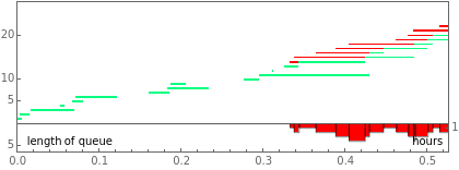
In the Demonstration graphic, the number of people in the queue is indicated by the height of the red bars at the bottom; the horizontal green lines indicate customers being served; red lines indicate customers waiting. The table below the graphic shows the expected and observed values of several values associated with such a process. Note that the basic units are hours, but some of the parameters are given in minutes.
In order to look at a typical window of the queue situation, a certain percentage of the initial customers is ignored. This is controlled by the choice of the initial deletion ratio. If this is set to 0 then one sees a simulation that starts with the first customer that walks in the door. In that case, the number in the queue or the system will generally be less than the expected value, since the queue is smaller than the limiting value at the start. If the deletion ratio is set to, say, 0.5, then the graphic shown will start with the customer in the order where is the total number of customers. Regardless of deletions, the time starts at 0.
N/2
N
Details
Details
The first snapshot shows the situation starting from an empty queue (initial deletion ratio is 0) and with . In that case the queue builds up and then increases without bound. The last two snapshots use two servers, with and . The first 70% of the time interval is deleted, thus giving a more typical window on the queue formation process. Still there is a lot of variation in the size of the queue: in the first case the average number of people waiting is 0.57 while in the second it is 13. For more information, see[1] and[2].
λ=μ
λ=50
μ=30
References
References
[1] F. S. Hillier and G. J. Lieberman, Introduction to Operations Research, 8th ed., New York: McGraw-Hill, 2004, pp. 765–774.
[2] R. B. Chase, F. R. Jacobs, and N. J. Aquilano, Operations Management for Competitive Advantage, 10th ed., New York: McGraw-Hill, 2004.
[2] R. B. Chase, F. R. Jacobs, and N. J. Aquilano, Operations Management for Competitive Advantage, 10th ed., New York: McGraw-Hill, 2004.
External Links
External Links
Permanent Citation
Permanent Citation
Karl W. Heiner, Stan Wagon
"Simulating a Multiple Server Queue"
http://demonstrations.wolfram.com/SimulatingAMultipleServerQueue/
Wolfram Demonstrations Project
Published: August 9, 2011