ABSTRACT (original article): The existence of solitons -- stable, long-lived, and localized field configurations -- is a generic prediction for ultralight dark matter. These solitons, known by various names such as boson stars, axion stars, oscillons, and Q-balls depending on the context, are typically treated as distinct entities in the literature. This study aims to provide a unified perspective on these solitonic objects for real or complex, scalar or vector dark matter, considering self-interactions and nonminimal gravitational interactions. We demonstrate that these solitons share universal nonrelativistic properties, such as conserved charges, mass-radius relations, stability and profiles. Without accounting for alternative interactions or relativistic effects, distinguishing between real and complex scalar dark matter is challenging. However, self-interactions differentiate real and complex vector dark matter due to their different dependencies on the macroscopic spin density of dark matter waves. Furthermore, gradient-dependent nonminimal gravitational interactions impose an upper bound on soliton amplitudes, influencing their mass distribution and phenomenology in the present-day universe. CITATION (original article): Hong-Yi Zhang, Unified view of scalar and vector dark matter solitons, arXiv:2406.05031. https://doi.org/10.48550/arXiv.2406.05031
Installation
Installation
Install the package “DMSolidonFinder” from https://github.com/hongyi18/DMSolitonFinder/ or follow the steps below:
Method 1: One can directly import the package from the web every time, using
Import["https://raw.githubusercontent.com/hongyi18/DMSolitonFinder/main/DMSolitonFinder.wl"]
Method 2: Download the package to the Applications subdirectory of $UserBaseDirectory, using
URLDownload["https://raw.githubusercontent.com/hongyi18/DMSolitonFinder/main/DMSolitonFinder.wl",FileNameJoin[{$UserBaseDirectory,"Applications","DMSolitonFinder.wl"}]]
To load the package, simply run
In[]:=
<<"DMSolitonFinder`"
DMSolitonFinder 1.0 has been loaded.
Basic usage
Basic usage
1. Set the value of the self-interaction (SI) coupling, nonminimal gravitational interaction (NGI) coupling, and polarization number/particle spin.
2. Choose the central amplitude of the soliton profile.
3. Use ShootFields.
2. Choose the central amplitude of the soliton profile.
3. Use ShootFields.
In[]:=
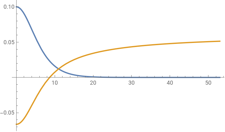
λ=1;(*SIcoupling.*)ξ=-1;(*NGIcoupling.*)σ=1;(*Polarizationnumber/particlespin.*)fi=1/10;(*Centralamplitudeofthesoliton.*)ri=;(*Locationoftheinnerboundary;defaultvalueis.*){sols,rf}=ShootFields[fi,SI->λ,NGI->ξ,Spin->σ];Plot[{sols[[1]][r],sols[[2]][r]},{r,ri,rf},PlotRange->All](*Plotf[r]andΨ[r].*)
-7
10
-7
10
Out[]=
Calculate mass, radius, particle number, frequency (chemical potential) and energy.
In[]:=
CalMass[sols[[1]],rf,NGI->ξ]CalRadius[sols[[1]],rf,NGI->ξ]CalParticleNumber[sols[[1]],rf]μ=CalFrequency[sols[[2]],rf]CalEnergy[sols[[1]],sols[[2]],μ,rf,NGI->ξ]
Out[]=
6.89846
Out[]=
11.175
Out[]=
6.89846
Out[]=
0.0616555
Out[]=
-0.128052
Advanced usage
Advanced usage
Print the Schroedinger-Poisson equations and the mass density .
ρ
ξ
In[]:=
Eqf[f,Ψ,r,SI->λ,NGI->ξ,Spin->σ]EqPsi[f,Ψ,r,NGI->ξ]MassDensity[f,r,NGI->ξ]
Out[]=
3
f[r]
12
1
2
2[r]
′
f
r
′′
f
2
f[r]
2
′
f
2[r]
′
f
r
′′
f
Out[]=
2
f[r]
2[r]
′
Ψ
r
2
′
f
2[r]
′
f
r
′′
f
′′
Ψ
Out[]=
2
f[r]
2
′
f
2[r]
′
f
r
′′
f
The field equations can be numerically solved using SolveFields.
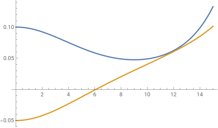
Example: Given the boundary values of f[r] and Ψ[r] at r=ri, solve the field equations between r=ri and r=rf with the Runge-Kutta method.
Example: Given the boundary values of f[r] and Ψ[r] at r=ri, solve the field equations between r=ri and r=rf with the Runge-Kutta method.
In[]:=
fi=1/10;Ψi=-5/100;ri=;rf=15;sols=SolveFields[fi,Ψi,rf,SI->λ,NGI->ξ,Spin->σ,MinRadius->ri,Method->"ExplicitRungeKutta"];(*Plotthefieldf[r]andΨ[r],whicharesols[[1]][r]andsols[[2]][r]respectively.*)Plot[{sols[[1]][r],sols[[2]][r]},{r,ri,rf}]
-8
10
Out[]=
For more details about the function, check the usage message by running “?FunctionName”.
In[]:=
?SolveFields
Out[]=
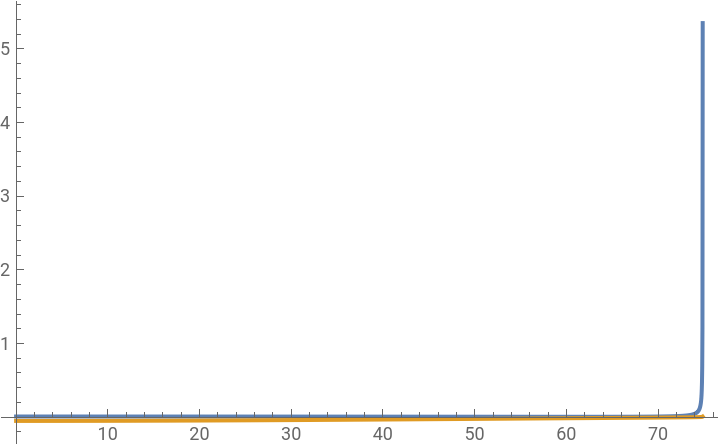
If ShootFields fails to find soliton profiles, try changing the default options.
In[]:=
λ=5000;(*SIcoupling.*)ξ=0;(*NGIcoupling.*)σ=0;(*Polarizationnumber/particlespin.*)fi=9/1000;(*Centralamplitudeofthesoliton.*)ri=;(*Locationoftheinnerboundary;defaultvalueis.*){sols,rf}=ShootFields[fi,SI->λ,NGI->ξ,Spin->σ,Method->"ExplicitRungeKutta"];Plot[{sols[[1]][r],sols[[2]][r]},{r,ri,rf},PlotRange->All](*Plotf[r]andΨ[r].*)
-7
10
-7
10
For fi=, increasing rf doesn't improve results after 84 calculations, relative amplitude at large radius is 594.547.
9
1000
Out[]=
Adjust the value of the option “FirstMinimumLocationRatio” might help:
In[]:=
λ=5000;(*SIcoupling.*)ξ=0;(*NGIcoupling.*)σ=0;(*Polarizationnumber/particlespin.*)fi=9/1000;(*Centralamplitudeofthesoliton.*)ri=;(*Locationoftheinnerboundary;defaultvalueis.*){sols,rf}=ShootFieldsfi,SI->λ,NGI->ξ,Spin->σ,Method->"ExplicitRungeKutta",FirstMinimumLocationRatio->;Plot[{sols[[1]][r],sols[[2]][r]},{r,ri,rf},PlotRange->All](*Plotf[r]andΨ[r].*)
-7
10
-7
10
93
100
For more solutions to common problems in finding optimal soliton profiles, please check https://github.com/hongyi18/DMSolitonFinder.
An example of producing the mass-radius relation of solitons with self-interactions
An example of producing the mass-radius relation of solitons with self-interactions
Consider negative self-interaction couplings λ<0
Consider negative self-interaction couplings λ<0
Solve soliton profiles with different central amplitudes.
Solve the mass and radius for those soliton solutions.
Consider positive self-interaction couplings λ<0. Calculations are similar to those for λ<0
Consider positive self-interaction couplings λ<0. Calculations are similar to those for λ<0
First solve soliton solutions with radii that are very close to the minimum allowed value, whose details can be found in the paper.
These solutions are steep and hard to find; one has to try adjusting different options for best results.
These solutions are steep and hard to find; one has to try adjusting different options for best results.
Then solve soliton solutions with larger radii.
Combine the results and make a plot for the mass-radius relation
Combine the results and make a plot for the mass-radius relation
CITE THIS NOTEBOOK
CITE THIS NOTEBOOK
DMSolitonFinder: package to solve dark matter soliton profiles
by Hong-Yi Zhang
Wolfram Community, STAFF PICKS, July 2, 2024
https://community.wolfram.com/groups/-/m/t/3203564
by Hong-Yi Zhang
Wolfram Community, STAFF PICKS, July 2, 2024
https://community.wolfram.com/groups/-/m/t/3203564