ABSTRACT (original article): The characterization of a quantum device is a crucial step in the development of quantum experiments. This is accomplished via Quantum Process Tomography, which combines the outcomes of different projective measurements to deliver a possible reconstruction of the underlying process. The tomography is typically performed by processing an overcomplete set of measurements and extracting the process matrix from maximum-likelihood estimation. Here, we introduce Fourier Quantum Process Tomography, a technique which requires a reduced number of measurements, and benchmark its performance against the standard maximum-likelihood approach. Fourier Quantum Process Tomography is based on measuring probability distributions in two conjugate spaces for different state preparations and projections. Exploiting the concept of phase retrieval, our scheme achieves a complete and robust characterization of the setup by processing a near-minimal set of measurements. We experimentally test the technique on different space-dependent polarization transformations, reporting average fidelities higher than 90% and significant computational advantage. CITATION (original article): Di Colandrea, F., Dehghan, N., D’Errico, A. et al. Fourier Quantum Process Tomography. npj Quantum Inf 10, 49 (2024). https://doi.org/10.1038/s41534-024-00844-7
1D Fourier Quantum Process Tomography
Data files are available at: https://github.com/FraDiColandrea/Fourier_Quantum_Process_Tomography
Experimental parameters
Experimental parameters
We set the physical parameters of our experiment, specifically the size of each pixel of our detection system (pixelsize), the spatial period Λ of our optical devices, and the number of pixels in a single period.
In[]:=
pixelsize=5.2*10^-6(*inmeters*);Λ=2.5*10^-3(*spatialperiod,inmeters*);
In[]:=
pixels=Round[Λ/pixelsize](*howmanypixelsinaperiod*)
Out[]=
481
Algorithm parameters
Algorithm parameters
We set the parameters of the Gerchberg-Saxton (GS) phase retrieval algorithm, specifically the number of global phase shifts to explore in the range [0,2π] (see Eqs. (5)-(6) of the main paper), the number of independent executions, and the number of iterations within a single execution.
In[]:=
offsets=64(*globalshiftstoexplore*);globalphase=Subdivide[0,2N[Pi],offsets-1](*globaloffsetsforreconstructedphases*);trials=100(*howmanyindependentexecutionsoftheGSalgorithm*);iterations=1000(*howmanyiterationswithinasingleexecution*);
Import experimental data
Import experimental data
We import the polarimetric data ⟨H∣U∣H⟩, ⟨D∣U∣D⟩, and ⟨L∣U∣L⟩ from the one-dimensional experiment. The total probability distribution (probtot) is also imported to solve the phase ambiguity (see Eq. (7) of the main paper).
In[]:=
SetDirectory[NotebookDirectory[]<>"Data/1D"](*Filestringformattingmayneedtobechangeddependingonoperatingsystem*)
Out[]=
C:\Users\franc\Desktop\postdoc\research\QPT_GS\github - FQPT2\Data\1D
HHnear=Import["HH_near.txt","List"](*nearfield*);HHfar=Import["HH_far.txt","List"](*farfield*);
DDnear=Import["DD_near.txt","List"](*nearfield*);DDfar=Import["DD_far.txt","List"](*farfield*);
LLnear=Import["LL_near.txt","List"](*nearfield*);LLfar=Import["LL_far.txt","List"](*farfield*);
probtot=Import["far_total.txt","List"](*totalfarfield*);
HH
HH
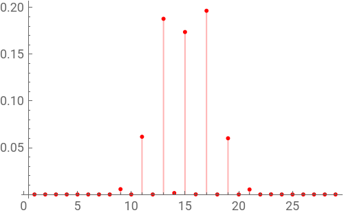
The phase retrieval algorithm is executed on the ⟨H∣U∣H⟩ measurement, taken in both the near field and the far field. The SU(2) parameters E and are extracted from Eqs. (6a)-(6b) using the best phase reconstruction, which is the one yielding the minimum error.
n
1
Phase retrieval
Phase retrieval
In[]:=
{ListPlot[HHnear,PlotStyle->Red,Joined->True,PlotRange->{0,1},ImageSize->250],ListPlot[HHfar,PlotRange->All,PlotStyle->Red,Joined->False,Filling->Axis,ImageSize->250]}
Out[]=
,
In[]:=
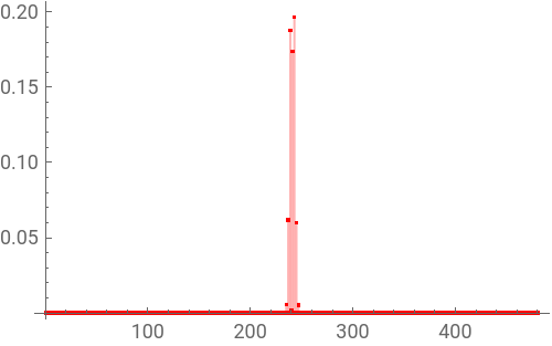
HHfar=ArrayPad[HHfar,(pixels-Length[HHfar])/2](*array-paddingneededforimplementingtheFFT*);
In[]:=
{ListPlot[HHnear,PlotStyle->Red,Joined->True,PlotRange->{0,1},ImageSize->250],ListPlot[HHfar,PlotRange->All,PlotStyle->Red,Joined->False,Filling->Axis,ImageSize->250]}
Out[]=
,
In[]:=
Dimensions[HHnear]==Dimensions[HHfar]
Out[]=
True
In[]:=
inputbeamHH=Sqrt[HHnear](*intensitytoamplitude*);outputbeamHH=RotateLeft[Sqrt[HHfar],(pixels-1)/2](*intensitytoamplitude,RotateLeftimplementstheFFTshiftcommand*);
In[]:=
error=Table[{},{i,trials}];phase=Table[{},{i,trials}];input=Table[{},{i,trials}];output=Table[{},{i,trials}];
In[]:=
(*RepeatedimplementationofGSalgorithm*)Monitor[Do[phaseguess=Table[RandomReal[{0,2N[Pi]}],{i,pixels}];inputGSguess=inputbeamHH*Exp[I*phaseguess];InputGS=inputGSguess;Do[outputGS=Fourier[InputGS,FourierParameters{0,1}](*FFT*);outputGS=outputGS*Sqrt[Total[Abs[outputbeamHH]^2]]/Sqrt[Total[Abs[outputGS]^2]];phaseoutputGS=Arg[outputGS];OutputGS=outputbeamHH*Exp[I*phaseoutputGS];inputGS=Fourier[OutputGS,FourierParameters{0,-1}](*inverseFFT*);phaseinputGS=Arg[inputGS];inputGS=inputGS*Sqrt[Total[Abs[inputbeamHH]^2]]/Sqrt[Total[Abs[inputGS]^2]];AppendTo[error[[t]],Total[Abs[Abs[inputGS]-inputbeamHH]]];InputGS=inputbeamHH*Exp[I*phaseinputGS];,{s,iterations}];phase[[t]]=phaseinputGS;input[[t]]=inputGS;output[[t]]=outputGS;,{t,trials}],{t,s}]
In[]:=
min=Flatten[Position[error[[All,-1]],Min[error[[All,-1]]]]][[1]];ListPlot[error[[min]]/Max[error],PlotRange->{0,1}]
Out[]=
In[]:=
inputGSHH=input[[min]];outputGSHH=output[[min]];phaseGSHH=phase[[min]];
In[]:=
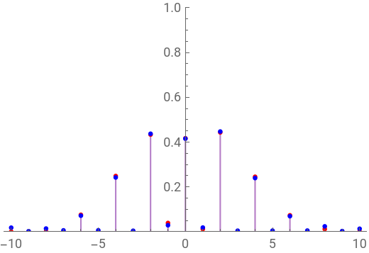
{ListPlot[{Abs[inputbeamHH],Abs[inputGSHH]},PlotRange->{0,1},PlotStyle->{Red,Blue},Joined->True,ImageSize->250],w=10;ListPlot[{RotateRight[Abs[outputbeamHH],(pixels-1)/2][[(pixels+1)/2-w;;(pixels+1)/2+w]],RotateRight[Abs[outputGSHH],(pixels-1)/2][[(pixels+1)/2-w;;(pixels+1)/2+w]]},DataRange->{-w,w},PlotRange->{0,1},PlotStyle->{Red,Blue},Joined->False,Filling->Axis,ImageSize->250,PlotLegends->{"Exp.","GS"}]}
Out[]=
,


Extracting SU(2) parameters
Extracting SU(2) parameters
PhaseGSHH=Table[Mod[phaseGSHH+globalphase[[i]],2N[Pi]],{i,offsets}];eGSHH=Table[ArcCos[inputbeamHH*Cos[PhaseGSHH[[i]]]],{i,offsets}](*globalphase-dependentretrievedE*);n1GS=Table[-inputbeamHH*Sin[PhaseGSHH[[i]]]/(Sin[eGSHH[[i]]]),{i,offsets}](*globalphase-dependentretrieved*);
n
1
In[]:=
Manipulate[{ListPlot[PhaseGSHH[[i]],Joined->False,PlotRange->{0,2N[Pi]},PlotStyle->Black,ImageSize200],ListPlot[eGSHH[[i]],PlotStyle->Red,PlotLegends->Automatic,Joined->True,PlotRange->{0,N[Pi]},ImageSize->200],ListPlot[n1GS[[i]],PlotStyle->Blue,PlotLegends->Automatic,Joined->True,PlotRange->{-1,1},ImageSize->200]},{i,1,offsets,1}](*thisallowsdynamicallyplottingthenon-equivalentparameterreconstructionsassociatedwithdifferentglobalshifts*);
DD
DD
Phase retrieval
Phase retrieval
Extracting SU(2) parameters
Extracting SU(2) parameters
LL
LL
Phase retrieval
Phase retrieval
Extracting SU(2) parameters
Extracting SU(2) parameters
Matching the global phase
Matching the global phase
Finding the unitary
Finding the unitary
We use the total far-field measurement (probtot) to solve the global phase ambiguity (see Eq. (7) of the main paper).
Reconstructed parameters
Reconstructed parameters
Among all possible unitaries, the reconstructed operator is the one minimizing the distance with the measured far-field intensity .
2D Fourier Quantum Process Tomography
Data files are available at: https://github.com/FraDiColandrea/Fourier_Quantum_Process_Tomography
Experimental parameters
Experimental parameters
We set the physical parameters of our experiment, specifically the size of each pixel of our detection system (pixelsize), the spatial period Λ of our optical devices, and the number of pixels in a single period. Additionally, we set the integration window (integrationpixels) to average over experimental imperfections and optimize computational efficiency in the two-dimensional implementation.
Algorithm parameters
Algorithm parameters
We set the parameters of the Gerchberg-Saxton (GS) phase retrieval algorithm, specifically the number of global phase shifts to explore in the range [0,2π] (see Eqs. (5)-(6) of the main paper), the number of independent executions, and the number of iterations within a single execution.
Import experimental data
Import experimental data
We import the polarimetric data ⟨H∣U∣H⟩, ⟨D∣U∣D⟩, and ⟨L∣U∣L⟩ from the two-dimensional experiment. The total probability distribution (probtot) is also imported to solve the phase ambiguity (see Eq. (7) of the main paper).
HH
HH
Phase retrieval
Phase retrieval
Extracting SU(2) parameters
Extracting SU(2) parameters
DD
DD
Phase retrieval
Phase retrieval
Extracting SU(2) parameters
Extracting SU(2) parameters
LL
LL
Phase retrieval
Phase retrieval
Extracting SU(2) parameters
Extracting SU(2) parameters
Matching the global phase
Matching the global phase
Finding the unitary
Finding the unitary
We use the total far-field measurement (probtot) to solve the global phase ambiguity (see Eq. (7) of the main paper).
Reconstructed parameters
Reconstructed parameters
Among all possible unitaries, the reconstructed operator is the one minimizing the distance with the measured far-field intensity .
CITE THIS NOTEBOOK
CITE THIS NOTEBOOK
Fourier quantum process tomography
by Francesco Di Colandrea, Nazanin Dehghan, Alessio D’Errico & Ebrahim Karimi
Wolfram Community, STAFF PICKS, June 3, 2024
https://community.wolfram.com/groups/-/m/t/3187336
by Francesco Di Colandrea, Nazanin Dehghan, Alessio D’Errico & Ebrahim Karimi
Wolfram Community, STAFF PICKS, June 3, 2024
https://community.wolfram.com/groups/-/m/t/3187336