ABSTRACT (original article): We present a general solution and formulation framework to Bellman’s lost-in-a-forest problem. The forest boundary is known and may take any shape. The starting point and the orientation are unspecified. The transformation allows us to formulate this problem as a constrained minimization problem. We leverage discrete optimization and derive several nontrivial results consistent with those from previous papers. CITATION (original article): Zhipeng Deng, A General Solution to Bellman’s Lost-in-a-forest Problem, arXiv:2412.10686. https://doi.org/10.48550/arXiv.2412.10686
Weak form - given forest boundary of any shape, search/escape from one known point but orientation is unknown
Weak form - given forest boundary of any shape, search/escape from one known point but orientation is unknown
Continuous formulation
Continuous formulation
Solve by calculus of variation: EL equation with Lagrange multiplier for constraints
Search for one line/half plane with unit distance
Search for one line/half plane with unit distance
Adding Lagrange multipliers to the objective functional
In[]:=
H=++λ[t]*(x[t]*Cos[t]+y[t]*Sin[t]-1);
2
x'[t]
2
y'[t]
In[]:=
Needs["VariationalMethods`"]
Euler - Lagrange Equations
In[]:=
EulerEquations[H,{x[t],y[t],λ[t]},t]
Out[]=
Cos[t]λ[t]+[t](-[t][t]+[t][t])0,Sin[t]λ[t]+[t]([t][t]-[t][t])0,-1+Cos[t]x[t]+Sin[t]y[t]0
′
y
′
y
′′
x
′
x
′′
y
3/2
([t]+[t])
2
′
x
2
′
y
′
x
′
y
′′
x
′
x
′′
y
3/2
([t]+[t])
2
′
x
2
′
y
Substitution and simplification
In[]:=
((D[H,x[t]]-D[D[H,x'[t]],t])*Sin[t]-(D[H,y[t]]-D[D[H,y'[t]],t])*Cos[t])/.[t]->D,t,[t]->D,{t,2}//Simplify
′
x
1-Sin[t]y[t]
Cos[t]
′′
x
1-Sin[t]y[t]
Cos[t]
Out[]=
(Sec[t](Sin[t]-y[t])(Sec[t](-3+Cos[2t]+4Sin[t]y[t])[t]+4[t]+2(Sin[t]-y[t])[t]))2(+-2Tan[t]y[t](Sec[t]-[t])-2Sin[t]Tan[t][t]+[t])[t]+
′
y
2
′
y
′′
y
2
Tan[t]
2
Sec[t]
2
y[t]
′
y
′
y
2
′
y
2
′
y
2
(y[t]+Tan[t](-Sec[t]+[t]))
2
Sec[t]
′
y
It is clear that the solution contain two partsand
(Sin[t]-y[t])
Sec[t](-3+Cos[2t]+4Sin[t]y[t])()[t]+4+2(Sin[t]-y[t])()[t]
′
y
2
()[t]
′
y
′′
y
Numerical solution using Finite Difference method to solve above EL equations
Numerical solution using Finite Difference method to solve above EL equations
Discretization points
In[]:=
pts=10002;
In[]:=
aa=N@Range[0,2π,2π/(pts-1)];grid=Flatten[Outer[List,aa],1];
Finite difference method
In[]:=
opt="DifferenceOrder"4;dfda=NDSolve`FiniteDifferenceDerivative[{1},{aa},opt]["DifferentiationMatrix"];d2fda2=NDSolve`FiniteDifferenceDerivative[{2},{aa},opt]["DifferentiationMatrix"];
In[]:=
nL=Length[grid];varsY=Table[Unique[y$],{aa}];
Approximate segmentation for EL equation
In[]:=
eqns=(Sec[aa](-3+Cos[2aa]+4Sin[aa]varsY)(dfda.varsY)+4+2(Sin[aa]-varsY)(d2fda2.varsY))*(Boole[0<=#<1.0472]&/@aa)+(Sin[aa]-varsY)*(Boole[1.0472<=#<3π/2]&/@aa)+(Sec[aa](-3+Cos[2aa]+4Sin[aa]varsY)(dfda.varsY)+4+2(Sin[aa]-varsY)(d2fda2.varsY))*(Boole[3π/2<=#<=2π]&/@aa);
2
(dfda.varsY)
2
(dfda.varsY)
In[]:=
eqns[[1]]=varsY[[1]]-0.57735;(*Approximateboundaryvalue*)eqns[[nL]]=varsY[[nL]]+1;
In[]:=
govEq=eqns;allVars=varsY;root=FindRoot[govEq,Thread[{allVars,Flatten[{Table[1,nL]}]}]];
Solve discretized equation
In[]:=
sol=allVars/.root;{ysoltemp}=Partition[sol,nL];ysol=Interpolation[Transpose[{aa,ysoltemp}]];
In[]:=
Plot,ysol[a],{a,0,2π},PerformanceGoal->"Speed",PlotRange->All,PlotLegends->{"x[a]","y[a]"}
1-Sin[a]ysol[a]
Cos[a]
Out[]=


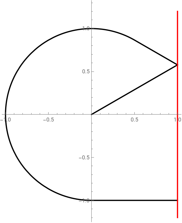
Boundary and path
In[]:=
ShowListLinePlot{0,0},,ysol[0],AspectRatio->Automatic,PerformanceGoal->"Speed",PlotRange->All,PlotStyle->Black,ParametricPlot,ysol[a],{a,0,2π},PerformanceGoal->"Speed",PlotRange->{{-1.5,1.5},{-1.5,1.5}},PlotStyle->Black,ContourPlot[x-1==0,{x,-1.2,1.2},{y,-1.2,1.2},ContourStyle->Red,PerformanceGoal->"Speed"],PlotRange->All,ImageSize->300
1-Sin[0]ysol[0]
Cos[0]
1-Sin[a]ysol[a]
Cos[a]
Out[]=
Length of path
In[]:=
2
1-Sin[0]ysol[0]
Cos[0]
2
ysol[0]
2
D,a
1-Sin[a]ysol[a]
Cos[a]
2
ysol'[a]
Out[]=
6.39724
The result consists of line segments and circular arcs . It was obtained and discussed in previous papers, but with geometric - based methodsThe exact solution is +1+
7π
6
3
Discrete formulation
Discrete formulation
Solve by function NMinimize
Search a line with unit distance
Search a line with unit distance
Number of discretization points
n=5000;
Numerical minimization for global optimal
sol=NMinimize++Sum+,{i,1,n}(*objective*),Tablex[i]*Cos*i+y[i]*Sin*i-1==0,{i,0,n}(*constraints*),Flatten[Table[{x[i],y[i]},{i,0,n}]];
2
x[0]
2
y[0]
2
(x[i]-x[i-1])
2
(y[i]-y[i-1])
2π
n
2π
n
Length of path
In[]:=
sol[[1]]
Out[]=
6.39724
In[]:=
RealDigits[%]
Out[]=
{{6,3,9,7,2,4,1,9,9,7,3,3,0,7,9,3},1}
In[]:=
Show[ListLinePlot[Prepend[Table[{x[i],y[i]},{i,0,n}]/.sol[[2]],{0,0}],AspectRatio->Automatic,PerformanceGoal->"Speed",PlotRange->All,PlotStyle->Black],ContourPlot[x-1==0,{x,-1.2,1.2},{y,-1.2,1.2},ContourStyle->Red,PerformanceGoal->"Speed"],PlotRange->All,ImageSize->300]
Out[]=
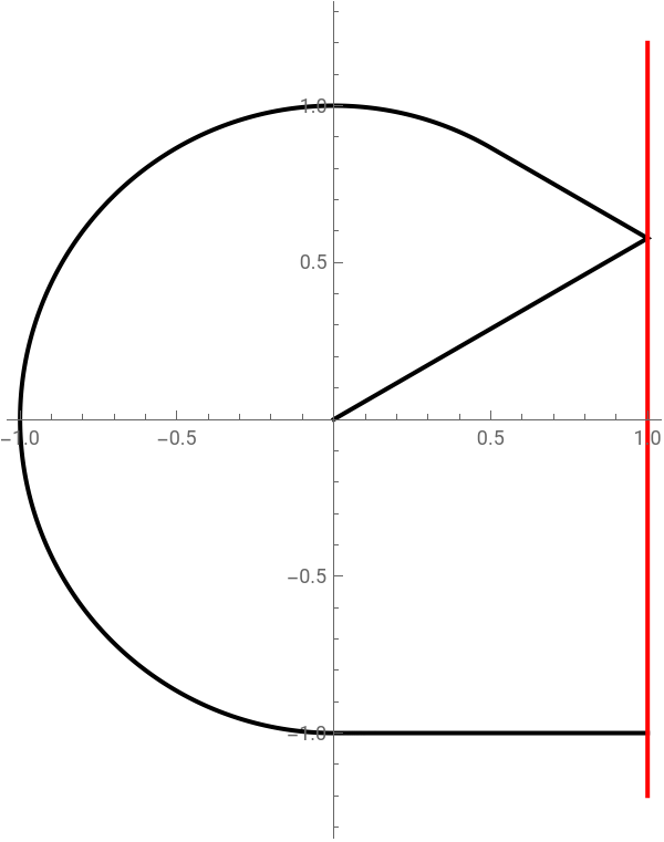
The result consists of line segments and circular arcs
Search a circle from exterior
Search a circle from exterior
Number of discretization points
Numerical minimization for global optimal
Length
The result consists of line segments and circular arcs
Search a circle from interior
Search a circle from interior
Number of discretization points
Numerical minimization for global optimal
Length
The result consists of line segments and circular arcs
Search a circle from interior when shortest path is not unique
Search a circle from interior when shortest path is not unique
Number of discretization points
Numerical minimization for global optimal
Length
Diameter 2 r = 3
The result consists of line segments and circular arcs
Search for one point with given distance 1
Search for one point with given distance 1
Number of discretization points
Numerical minimization for global optimal
Length
the length should be 2 π + 1
The result consists of line segments and circular arcs
The exact solution is 1 + 2 π
The exact solution is 1 + 2 π
Search for a shape from interior with distance significantly short at certain angle, when shortest path is not unique
Search for a shape from interior with distance significantly short at certain angle, when shortest path is not unique
Only search for circle
Number of discretization points
Numerical minimization for global optimal
only search for line segment
Search for circle and line segment
Shortest path is not unique, as length of both path is 1
Two perpendicular lines with 0.5 distance
Two perpendicular lines with 0.5 distance
The result consists of line segments and circular arcs
Two parallel lines from the middle
Two parallel lines from the middle
The result consists of line segments and circular arcs
Search for two lines from the angle bisector in the middle
Search for two lines from the angle bisector in the middle
π/6 - 30 degree
π/3 - 60 degree
2 π/3 - 120 degree
5 π/6 - 150 degree
Search for two parallel lines with unit distance (unit strip) from one line
(Zalgaller class 2)
Search for two parallel lines with unit distance (unit strip) from one line
(Zalgaller class 2)
(Zalgaller class 2)
The result consists of three line segments and one circular arc
CITE THIS NOTEBOOK
CITE THIS NOTEBOOK
A general solution to Bellman's lost-in-a-forest problem
by Zhipeng Deng
Wolfram Community, STAFF PICKS, January 9, 2025
https://community.wolfram.com/groups/-/m/t/3354210
by Zhipeng Deng
Wolfram Community, STAFF PICKS, January 9, 2025
https://community.wolfram.com/groups/-/m/t/3354210