Reading the map. The green line is the equatorward edge of the auroral oval — aurora is overhead poleward of it and (a little) on the horizon just equatorward. It looks tilted and wavy because the oval circles the geomagnetic pole (over Arctic Canada, not the geographic pole). The orange dashed curve is the day/night line (aurora is only visible on the dark side); the yellow dot is where the Sun is overhead.
This notebook is a complete, runnable space-weather tool. It streams the live solar wind measured by NASA/NOAA’s DSCOVR spacecraft at the L1 Lagrange point and turns it, through physics implemented from scratch, into a planetary-Kp nowcast, a ring-current (Dst) forecast, a global auroral-oval map, and a location-aware visibility forecast for anywhere on Earth — complete with tonight’s darkness window, the Moon, and a plain-language verdict. It cross-checks against NOAA’s authoritative OVATION aurora model and the AuroraWatch UK magnetometer, and the whole thing is wrapped in an interactive dashboard that is deployed to the Wolfram Cloud as a web API, a web form, and an interactive app. All logic lives in a single package, AuroraMonitor.wl, loaded below; every figure is produced by the visible call printed above it. Live at build time: Kp 1.3, solar wind 426. km/s, Bz 0.9 nT.
As a taste of what the tool draws, here is the global auroral oval expanding equatorward over both hemispheres as the storm level climbs from quiet to severe (Kp 09). The whole animation is one call:
1. Setup: one package, every live feed
1. Setup: one package, every live feed
Everything is in one self-contained package, AuroraMonitor.wl, which ships in the same folder as this notebook. Loading it brings in the physics, the live data fetchers, the maps, the location engine and the dashboard:
SetDirectory[NotebookDirectory[]];Get["AuroraMonitor.wl"];Needs["AuroraMonitor`"];
A single call fetches every live feed — DSCOVR solar wind, planetary Kp (now and the 3-day forecast), Kyoto Dst, the NOAA G/S/R storm scales, F10.7 flux, GOES X-rays, the OVATION aurora grid, and AuroraWatch UK — into one association:
data=auroraData[];
Here is the current state of the heliosphere as a live gauge strip (each chip is computed from data):
gaugeStrip[spaceWeatherSummary[data]]

2. The Sun, the solar wind, and the coupling function
2. The Sun, the solar wind, and the coupling function
Everything starts at the Sun. Coronal holes blow the high-speed solar wind; sunspots and active regions store the magnetic energy that erupts as flares and coronal mass ejections. Here is the Sun right now — corona, chromosphere, surface magnetic field, and sunspots — straight from NASA's Solar Dynamics Observatory:
latestSolarImages[235]
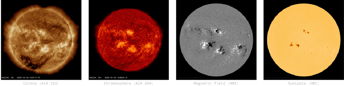
The Sun now (NASA SDO). Dark patches in the AIA 193 corona are coronal holes (fast-wind sources); the speckles in the HMI magnetic-field image are active regions, where flares and CMEs originate.
You can also build a time-lapse video of the Sun and choose how many days it spans — in the live notebook the slider and button below are interactive (the video downloads NASA imagery on demand):
solarExplorer[]
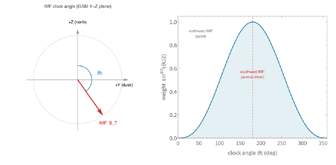
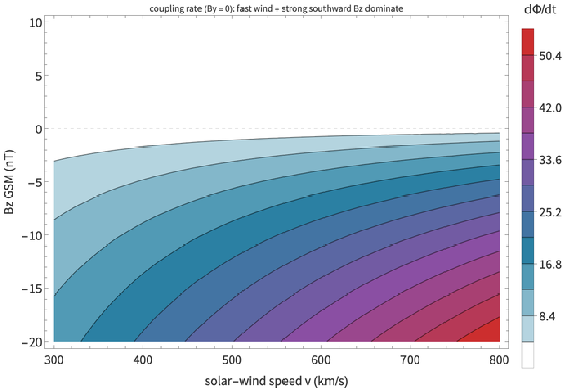
That solar activity, two to four days later, arrives at Earth as the solar wind. The aurora is powered by that wind opening magnetic flux at the dayside magnetopause. How fast that happens is captured by the Newell et al. (2007) coupling function, built from the wind speed v, the transverse interplanetary field Bt, and the clock angle θc (how far south the field points):
Φ
t
4/3
v
2/3
B
T
8
3
sin
θ
c
2
In code that is a one-liner, here evaluated on a strongly-southward example (fast wind, Bz = -12):
newellCoupling[650.,4.,-12.]
29526.1
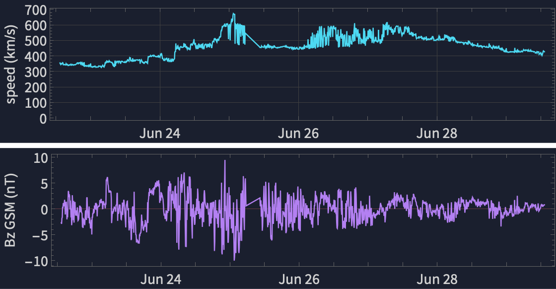
Run on every one-minute DSCOVR sample, it turns the messy wind into a single driving rate. The live 7-day record of speed and Bz (the southward excursions are the geo-effective ones):
solarWindPlot[data,560]
The clock-angle weighting and the full sensitivity of the coupling rate to speed and Bz (strongest for fast wind + strong southward field):
3. Kp now, and the 3-day forecast
3. Kp now, and the 3-day forecast
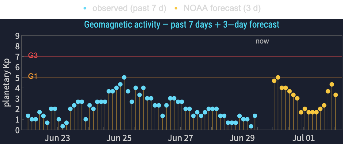
The planetary K-index is the 0–9 workhorse of aurora forecasting. We relate it to the time-averaged coupling rate through a transfer function calibrated against the live NOAA Kp feed, and we also ingest NOAA's official 3-day predicted Kp:
Kpa+b
p
S
lag
S
0
kpForecastPlot[data,560]
4. Storm intensity: the ring current (Dst)
4. Storm intensity: the ring current (Dst)
During a storm a westward ring current grows and depresses the surface field — the Dst index. We forecast it from DSCOVR with the Burton (1975) / O'Brien–McPherron (2000) injection–decay equation, driven by the rectified dawn–dusk field VBs:
"*"
Dst
t
"*"
Dst
τ(VBs)
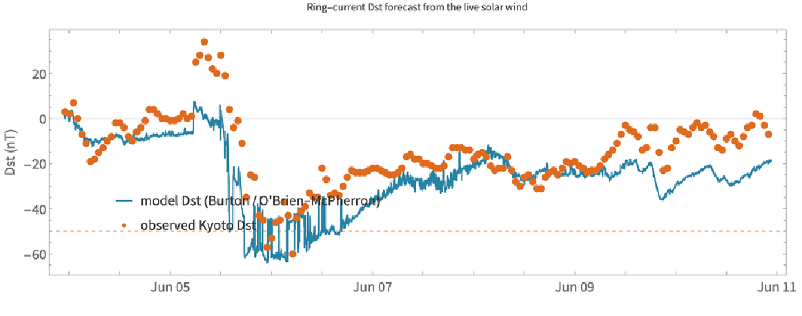
The model and the live Kyoto Dst over the past week (our model in teal):
With[{sw=data["solarWind"]},integrateDst[#time&/@sw,#speed&/@sw,#density&/@sw,#bz&/@sw,First[data["dst"]["dst"]]]//Last//Take[#,-3]&]
{-11.8618,-12.3058,-12.2491}
(the latest three modelled Dst values, nT). Integrated over the whole week the model tracks the observed Kyoto Dst through the storm, including the dynamic-pressure spike at stream arrival:
5. Where the oval sits: geomagnetic latitude
5. Where the oval sits: geomagnetic latitude
6. The global auroral oval
6. The global auroral oval
With the geomagnetic geometry in hand we can draw the auroral oval over the whole Earth — both hemispheres — together with the day/night terminator and a location pin. Here at a moderate Kp = 6 storm, pinned on Fairbanks:
Green = oval edge (aurora overhead poleward of it); orange dashed = day/night line (aurora only on the dark side); yellow dot = Sun overhead; red dot = the chosen location. The oval is tilted/wavy because it rings the geomagnetic pole over Arctic Canada, not the geographic pole.
7. Cross-checks: OVATION, AuroraWatch UK & ground magnetometers
7. Cross-checks: OVATION, AuroraWatch UK & ground magnetometers
Our oval is a clean physical model; NOAA's OVATION assimilation is the authoritative live nowcast. We overlay ours (white dashed) on theirs (colour = aurora probability) — a model-vs-data validation in one picture:
A second, independent check on the ground: AuroraWatch UK (Lancaster University) runs a magnetometer at Crooktree in Aberdeenshire and issues a green/yellow/amber/red alert from the measured field disturbance. Its hourly activity and the planetary Kp over the same window tell one consistent story:
And we can look at the raw magnetometer traces themselves. Pulling the actual ground-field records from three UK observatories (INTERMAGNET / BGS) and stacking them by latitude shows the key fact behind the whole tool: the same disturbance is bigger and sharper the further north you are (closer to the auroral electrojet) — Lerwick (Shetland) swings hardest, Hartland least:
Ground magnetometers (INTERMAGNET / BGS). Horizontal-field disturbance ΔX at Lerwick (60°N), Eskdalemuir (55°N) and Hartland (51°N), stacked. The open archive lags real time by ~1–2 weeks, so this is the most recent published window; the live ground truth above is AuroraWatch UK.
8. Regional visibility maps
8. Regional visibility maps
For any region, a dark-sky map shades the sky by how high the aurora would sit above the northern horizon — brighter green means higher and more likely seen. Alaska at Kp = 6:
The same one call works for Scotland, the Nordic countries, the Great Lakes, or any {{latmin,latmax},{lonmin,lonmax}}. Here is Scotland at three storm levels — at Kp 8 the oval is overhead across the whole country:
Figures. Horizon geometry of the emission layer, and aurora elevation vs corrected geomagnetic latitude for several Kp (these two are rendered by wolfram/oval.wls).
9. Your location: a personal forecast
9. Your location: a personal forecast
The heart of the tool. Give it any city in the world (or {lat, lon}) and the current Kp, and it returns the geomagnetic latitude, the Kp thresholds for overhead and horizon aurora, tonight's astronomical darkness window, the Moon, and a plain-language verdict:
Note how the engine is honest about viewing conditions: at high latitude near midsummer it will tell you the sky never gets dark. As JSON (this is exactly what the deployed web API returns):
10. The interactive dashboard
10. The interactive dashboard
All of the above is wrapped into one interactive explorer with six views — Now, Location, Explore Kp, Global map, Solar wind and Space weather. In the live notebook this is fully interactive; the screenshot below is its Now view — gauges, the go/no-go verdict, the global oval, and the planetary-Kp activity for the past week plus the 3-day forecast. Evaluate the call below to drive it yourself (it reuses the data fetched above). Each view re-renders the maps, so allow a couple of seconds after every click.
11. Deploying it to the cloud
11. Deploying it to the cloud
Because the package is self-contained, the same functions deploy to the Wolfram Cloud unchanged. A web API that anyone (or any program) can call:
For the browser, the dashboard deploys as a server-rendered form (pick a view, a location and a what-if Kp, click Submit, and it renders that view live from DSCOVR — reliably, in ~10–25 s, with the browser's loading spinner). The fully live, instant single-page explorer (auroraExplorer[]) runs best in a desktop session; cloud interactive apps render too slowly for a good experience. The build script is wolfram/deploy.wls. Live endpoints: API, web form, explorer (currently private to the author).
This is the Space weather view of the deployed dashboard — the solar drivers and storm scales, the planetary-Kp history and 3-day forecast, and the ring-current (Dst) storm history:
12. What it can and cannot do
12. What it can and cannot do
• Lead time is short. DSCOVR buys ~30–60 minutes (the L1 advection time), not days.
• The Kp transfer is deliberately simple — a transparent fit, not the operational Wing (2005) network.
• Our oval is a boundary, not a brightness model; for authoritative live probability we defer to OVATION (§7).
• Geomagnetic coordinates are approximated by a centred dipole with a fixed regional correction (~1°).
• Clouds and daylight still win — the tool reports darkness and Moon, but not local weather.
13. References
13. References
• Newell, P. T., et al. (2007). A nearly universal solar wind–magnetosphere coupling function. J. Geophys. Res. 112, A01206.
• Burton, R. K., R. L. McPherron, C. T. Russell (1975). An empirical relationship between interplanetary conditions and Dst. J. Geophys. Res. 80, 4204.
• O'Brien, T. P., R. L. McPherron (2000). Empirical phase-space analysis of ring-current dynamics. J. Geophys. Res. 105, 7707.
• Newell, P. T., et al. (2014). OVATION Prime aurora model. Space Weather 12, 368.
• Shepherd, S. G. (2014). Altitude-adjusted corrected geomagnetic coordinates (AACGM-v2). J. Geophys. Res. Space Physics 119, 7501.
• World Data Center for Geomagnetism, Kyoto (Dst), via NOAA SWPC.
• INTERMAGNET and the British Geological Survey (ground-magnetometer data, Lerwick / Eskdalemuir / Hartland): intermagnet.org.
• NASA / SDO (Solar Dynamics Observatory imagery, courtesy of NASA/SDO and the AIA, EVE and HMI science teams; the SolarVideo resource function): sdo.gsfc.nasa.gov.
14. Acknowledgements
14. Acknowledgements
Data from NOAA SWPC (DSCOVR, Kp, OVATION, scales, GOES; US Government work, public domain) and the World Data Center for Geomagnetism, Kyoto (Dst). The ground-magnetic alert status is from AuroraWatch UK (non-commercial use), derived from the Sub-Auroral Magnetometer Network (SAMNET), operated by the Space and Plasma Physics group, Lancaster University (© Lancaster University). The ground-magnetometer traces rely on data collected at the Lerwick, Eskdalemuir and Hartland observatories: we thank the British Geological Survey for operating them and INTERMAGNET for promoting high standards of magnetic observatory practice (intermagnet.org); these reported data are licensed CC BY-NC 4.0 and used here for non-commercial, scientific purposes with attribution. Formal citation and DOIs for the definitive BGS observatory data are available from the BGS geomagnetism data service (geomag.bgs.ac.uk) and the World Data Centre for Geomagnetism, Edinburgh. Solar imagery is courtesy of NASA/SDO and the AIA, EVE and HMI science teams. All numerics, geodesy, maps and the cloud deployment are pure Wolfram Language. The repository scaffold and build pipeline were prepared with the help of Anthropic's Claude Code.
15. Reproducibility
15. Reproducibility
The entire project is one package plus thin scripts. To run the tool yourself:
Get["wolfram/AuroraMonitor.wl"]; Needs["AuroraMonitor`"];
auroraExplorer[] (* live interactive dashboard *)
locationForecast["Edinburgh", 6.0] (* any location on Earth *)
(* deploy your own copy: *)
wolframscript -file wolfram/deploy.wls
auroraExplorer[] (* live interactive dashboard *)
locationForecast["Edinburgh", 6.0] (* any location on Earth *)
(* deploy your own copy: *)
wolframscript -file wolfram/deploy.wls
Generated June 29, 2026 from live data.
CITE THIS NOTEBOOK
CITE THIS NOTEBOOK
Aurora monitor: a real-time space-weather and aurora-visibility dashboard
by Marco Thiel
Wolfram Community, STAFF PICKS, June 29, 2026
https://community.wolfram.com/groups/-/m/t/3741265
by Marco Thiel
Wolfram Community, STAFF PICKS, June 29, 2026
https://community.wolfram.com/groups/-/m/t/3741265