Steady Potential Flow through Box with Staggered Inlet and Outlet
Authors: Housam Binous and Ahmed Bellagi
Steady Potential Flow through Box with Staggered Inlet and Outlet
Authors: Housam Binous and Ahmed Bellagi
Authors: Housam Binous and Ahmed Bellagi
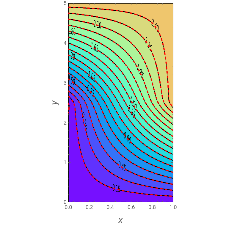
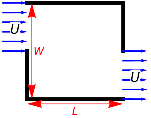
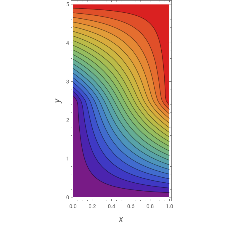
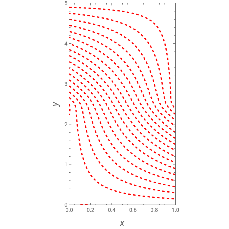
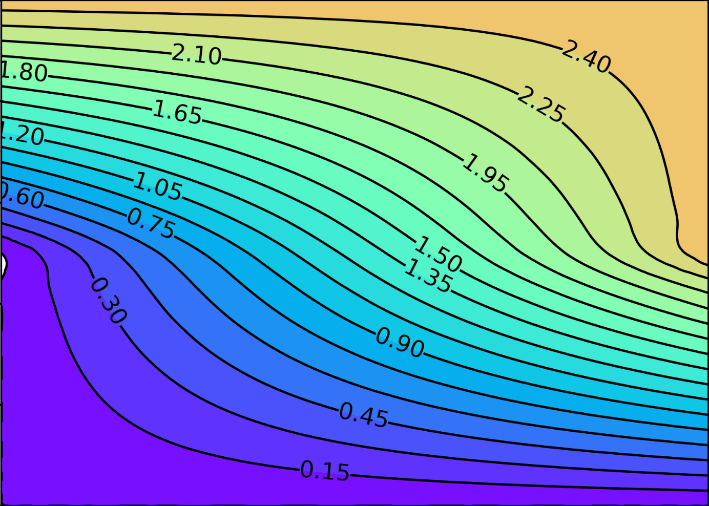
Consider the flow through a two-dimensional box with staggered inlet and outlet as show in the figure below:The flow enters and exits the box with a uniform speed . The aspect ratio of the box is =0.2.We plot the streamlines for this potential flow for a user-set value of .These streamlines are the solution of the equation ψ+ψ=0 subject to the boundary conditions:BC1: at , for and for ,BC2: at , for and for ,BC3: at , for , andBC4: at , for .The solution methodology, thoroughly described in Ref. 1, is based on Chebyshev orthogonal collocation with collocation points.This problem also admits an analytical solution given by T. Bennett [2]:,where =nπ/W. We have found excellent agreement between our numerical solutions (with Mathematica and Python) and the analytical solution by Bennett.References:[1] H. Binous, S. Kaddeche and A. Bellagi, Solving two-dimensional chemical engineering problems using the chebyshev orthogonal collocation technique, Computer Applications in Engineering Education, 24(1), pp. 144-155, 2016. https://onlinelibrary.wiley.com/doi/abs/10.1002/cae.21680[2] T. Bennett, Transport by Advection and Diffusion, New York: Wiley, 2012.
U=1
γ=L/W
γ
2
∂
∂
2
x
2
∂
∂
2
y
x=0
ψ=0
0⩽y≤W/2
ψ=U(y-W/2)
W/2⩽y≤W
x=L
ψ=Uy
0⩽y≤W/2
ψ=UW/2
W/2⩽y≤W
y=0
ψ=0
0⩽x≤L
y=L
ψ=UW/2
0⩽x≤L
N=31
ψ=Uy/2+2UW(sinh(x)-sinh((L-x)))sin(y)
∞
∑
n=1
2
λ
n
sin(nπ/2)
sinh(L)
λ
n
λ
n
λ
n
λ
n
λ
n
In[]:=
L=1;Ua=1;lamda[n_]:=nPi/W;gamma=0.2;
In[]:=
Np=30;Ds=Table[d[i,j],{i,0,Np},{j,0,Np}];d[0,0]=(2Np^2+1)/6//N;d[Np,Np]=-(2Np^2+1)/6//N;d[i_,i_]:=-y[i]/(2(1-y[i]^2));y[i_]:=Cos[iPi/Np]//N;d[j_,k_]:=If[j≠k,c[j](-1)^(j+k)/(c[k](y[j]-y[k]))];c[i_]:=If[i0||iNp,2,1];Dsq=Ds.Ds;L2b=4KroneckerProduct[IdentityMatrix[Np+1],Dsq];x1=Table[1/2(1+y[i]),{i,Np,0,-1}];W=L/gamma;L2a=4gamma^2KroneckerProduct[Dsq,IdentityMatrix[Np+1]];x2=Table[1/(2gamma)(1+y[i]),{i,Np,0,-1}];
In[]:=
U=Table[u[i+(j-1)(Np+1)],{j,1,Np+1},{i,1,Np+1}]//Flatten;Eq[i_]:=L2a[[i]].U+L2b[[i]].U0;bc1a=Table[u[1+(j-1)(Np+1)]0,{j,1,15}];bc1b=Table[u[1+(j-1)(Np+1)]Ua(x2[[j]]-W/2.),{j,16,Np+1}];bc2a=Table[u[Np+1+(j-1)(Np+1)]Uax2[[j]],{j,1,15}];bc2b=Table[u[Np+1+(j-1)(Np+1)]UaW/2.,{j,16,Np+1}];bc3=Table[u[i]0,{i,2,Np}];bc4=Table[u[i+Np(Np+1)]UaW/2.,{i,2,Np}];sys=Join[{bc1a,bc1b,bc2a,bc2b,bc3,bc4,Table[Eq[i+(j-1)(Np+1)],{j,2,Np},{i,2,Np}]}]//Flatten;initguess=Flatten[Table[{u[i+(j-1)(Np+1)],0.5},{j,1,Np+1},{i,1,Np+1}],1];sol=FindRoot[sys,initguess];a=Flatten[Table[{x1[[i]],x2[[j]],u[i+(j-1)(Np+1)]/.sol},{j,1,Np+1},{i,1,Np+1}],1];f=Interpolation[a,InterpolationOrder3];ContourPlot[f[x1,y1],{x1,0,1},{y1,0,1/gamma},FrameLabel{Style["x",Italic,16],Style["y",Italic,16]},PlotLegendsAutomatic,ColorFunction"Rainbow",Contours20,AspectRatio2,ImageSize380{1,1}]
Out[]=

In[]:=
p2=ContourPlot[f[x1,y1],{x1,0,1},{y1,0,1/gamma},FrameLabel{Style["x",Italic,16],Style["y",Italic,16]},PlotLegendsAutomatic,ColorFunction"Rainbow",ImageSize380{1,1},ContourShading->None,ContourStyle->{{Red,Dashed,Thick}},ContoursTable[i,{i,0.,3.5,0.15}],PlotRange->{{0,1},{0,5}},AspectRatio->1.9]
Out[]=
comparing the solutions obtained with Mathematica and Python
In[]:=
img=
;(*contourplotobtainedwithPython*)
In[]:=
Show[p2,Prolog->{Raster[ImageData[img,DataReversed->True],{Scaled[{0.0,0.0}],Scaled[{1,1}]}]},AspectRatio->1.9]
Out[]=