ORIGINAL ARTICLE: Minzhang Zheng, Richard Sear, Lucia Illari, Nicholas J. Restrepo, Neil F. Johnson, Adaptive link dynamics drive online hate networks and their mainstream influence, arXiv:2307.12559
DOI: https://doi.org/10.48550/arXiv.2307.12559
DOI: https://doi.org/10.48550/arXiv.2307.12559
Online hate is dynamic, adaptive and is now surging, armed with AI/GPT tools. Its consequences include personal traumas, child sex abuse, and violent mass attacks. Overcoming it will require knowing how it operates at scale. Here we present this missing science and show that it contradicts current thinking. Waves of adaptive links connect the hate user base over time across a sea of smaller platforms, allowing hate networks to steadily strengthen, bypass mitigations, and increase their direct influence on the massive neighboring mainstream. The data suggests 1 in 10 of the global population have recently been exposed, including children. We provide governing dynamical equations derived from first principles. A tipping-point condition predicts more frequent future surges in content transmission. Using the U.S. Capitol attack and a 2023 mass shooting as illustrations, we show our findings provide abiding insights and quantitative predictions down to the hourly scale. The expected impacts of proposed mitigations can now be reliably predicted for the first time.
Introduction
Introduction
The paper analyzes online hate network dynamics and their influence on the mainstream. It shows that hate networks exhibit adaptive linking behavior, connecting across platforms and directly to the mainstream in shock-like waves around events. It is this linking that allows hate networks to steadily strengthen over time, rather than remain on isolated fringes. A significant portion of the global population may have been recently exposed to online hate. The paper derives governing equations that mathematically reproduce the observed linking patterns. The solutions provide quantitative predictions for forecasting, evaluating mitigations, and guiding policy.
This notebook details the modeling work behind the equations. The empirical linking data is imported and prepared. The mathematical model assumptions are outlined. The model is fitted to real data for just prior to Jan. 6th 2021 and Jan. 6th itself, and predictions are compared back to the empirical data for validation. This notebook elucidates how the equations accurately capture real hate linkage pattern, and offers insights into harnessing the model to combat online hate. The notebook complements the broader study by detailing the modeling approach. Together, these works characterize online hate ecosystems to inform interventions.
This notebook details the modeling work behind the equations. The empirical linking data is imported and prepared. The mathematical model assumptions are outlined. The model is fitted to real data for just prior to Jan. 6th 2021 and Jan. 6th itself, and predictions are compared back to the empirical data for validation. This notebook elucidates how the equations accurately capture real hate linkage pattern, and offers insights into harnessing the model to combat online hate. The notebook complements the broader study by detailing the modeling approach. Together, these works characterize online hate ecosystems to inform interventions.
Data loading and preprocessing
Data loading and preprocessing
Define a function to convert hexadecimal color codes to RGB format and define a dictionary to map platforms to specific colors:
In[]:=
ClearAll["Global`*"];ClearSystemCache[];
In[]:=
hexToRGB=RGBColor@@(IntegerDigits[#~StringDrop~1~FromDigits~16,256,3]/255.)&;colors={"4Chan"->hexToRGB@"#fa776e","TG"->hexToRGB@"#649bf9","YouTube"->hexToRGB@"#ad2120","Twitter"->hexToRGB@"#ffd70a","Other"->Black}
Out[]=
{4Chan,TG,YouTube,Twitter,Other}

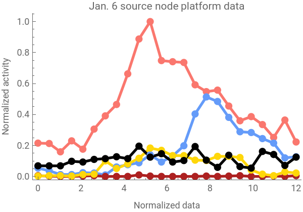
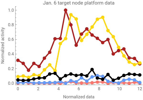
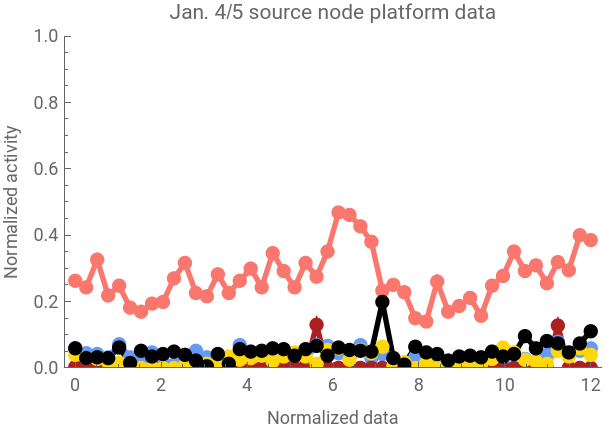
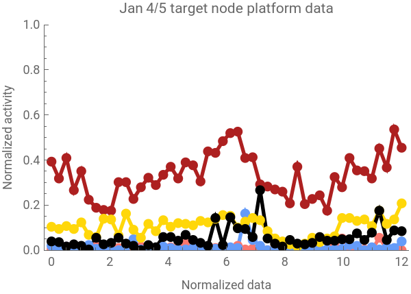
The empirical data was obtained by compressing fringe network data into hourly time series centered on January 6, 2021. Focus was placed on the top 4 most active platforms - 4Chan, Telegram, YouTube, and Twitter. The remaining platforms were aggregated as ‘Other’. In both cases, ‘Other’ represented significantly fewer links than the top platforms. The counts were normalized on a 0 to 1 scale and times converted to 0 to 12 range. This allows representing the platforms as variables Z, Y, X, W, V in the model (seen later in this notebook), with interaction terms tracking platform interconnections. The process can be repeated for additional platforms and dates, generating similar dynamical plots.
Import the dataset from a CSV file for Jan . 6th and Jan . 4 - 5 :
In[]:=
dJ6=Import[DirectoryName[NotebookDirectory[]]<>"data\\jan6_wide.csv","CSV"];dJ4=Import[DirectoryName[NotebookDirectory[]]<>"data\\jan_wide.csv","CSV"];(*Displaythefirsttworowsofeachdataset*)dJ6[[1;;2]]dJ4[[1;;2]]
Out[]=
{{created_at,type,4Chan,TG,YouTube,Twitter,Other},{2021-01-06 15:00:00,source,0.215159,0.0537897,0.00488998,0.00244499,0.0684597}}
Out[]=
{{created_at,type,4Chan,TG,YouTube,Twitter,Other},{2021-01-04 00:00:00,source,0.560209,0.125654,0.0052356,0.0837696,0.125654}}
Preprocess the ‘source’ and ‘target’ data: rescale the indices and join them with the corresponding data row. Here, the ‘source’ and ‘target’ data represent the linking activity between different communities on specific platforms. In this context, ‘source’ refers to the community where the link originates, and ‘target’ refers to the community where the link leads. The data is derived from an edge list, which is a common way to represent network data, and it provides a tally of the linking activity between these communities.
In[]:=
preprocessData[data_,dataType_,divideBy_:Automatic]:=Module[{selectedData=Select[data,#[[2]]==dataType&],rescaleFactor},rescaleFactor=If[divideBy===Automatic,Length@selectedData/2,Length@selectedData/divideBy];Transpose@Join[{Table[Rescale[i,{1,Length@selectedData},{0,rescaleFactor}],{i,Length@selectedData}]},Transpose@selectedData]]rescaleElements[data_,rescaleRange_]:=Table[Join[data[[i,1;;3]],Rescale[data[[i,4;;8]],{0,1},rescaleRange]],{i,Length@data}]
The Jan. 6th and Jan. 4-5th data is rescaled differently. For the Jan. 6th data, the indices are rescaled from their original range to a new range that is half the length of the selected data, and is done for both the ‘source’ and ‘target’ data. For the Jan. 4-5th data, the rescaling process involves adjusting the indices based on a calculated factor to match the conditions on Jan. 6th, and then further rescaling specific elements within each row of the ‘source’ and ‘target’ data to align with the maximum values observed on Jan. 6th.
In[]:=
sourceJ6=preprocessData[dJ6,"source"];targetJ6=preprocessData[dJ6,"target"];divideBy=Round[x/.First@Solve[((Length@dJ4-1)/2)/x==12,x]];sourceJ4=preprocessData[dJ4,"source",divideBy];targetJ4=preprocessData[dJ4,"target",divideBy];sourceREJ4=rescaleElements[sourceJ4,{0,192/410}];targetREJ4=rescaleElements[targetJ4,{0,166/310}];
Data visualization
Data visualization
The data is visualized using several plots, where each plot represents the' source' or' target' data, with each data point corresponding to a specific platform. The platforms are color-coded for easy identification.
createPlot[data_,plotLabel_,joined_:False,plotRange_:Automatic,xAxisLabel_:None,yAxisLabel_:None]:=ListPlot[Evaluate@Table[data[[All,{1,i}]],{i,4,8}],PlotStyle->Table[{Thickness[0.01],Values@colors[[i]]},{i,5}],Frame->{{True,False},{True,False}},FrameLabel->{{yAxisLabel,None},{xAxisLabel,None}},PlotLabel->plotLabel,PlotMarkers->Graphics@{Disk[{0,0},Scaled@0.02]},Joined->joined,ImageSize->Medium,PlotRange->plotRange]
In[]:=
Grid[{{createPlot[sourceJ6,"Jan. 6 source node platform data",True,Automatic,"Normalized data","Normalized activity"],createPlot[targetJ6,"Jan. 6 target node platform data",True,Automatic,"Normalized data","Normalized activity"]},{createPlot[sourceREJ4,"Jan. 4/5 source node platform data",True,{0,1},"Normalized data","Normalized activity"],createPlot[targetREJ4,"Jan 4/5 target node platform data",True,{0,1},"Normalized data","Normalized activity"]}}]
Out[]=
Model definition and simulation
Model definition and simulation
The online hate linking dynamics of five different platforms (Z, Y, X, W, V) are modeled using a system of differential equations. Key parameters account for the capacity, onset delay, growth and decay rates, and coupling between different platforms. The carrying capacity parameter represents the maximum population size a platform can sustain. Onset delay is the time before growth or decay begins for a platform. Growth and decay rates control how quickly the platform size increases or decreases. Coupling parameters quantify the inter-platform influence and feedback.
Intrinsic growth and decay are captured by self-interaction terms for each platform. Coupling terms reflect differences between platforms and can be positive (indicating amplification) or negative (indicating suppression). Interaction terms are only included where needed to improve model fit. Decay terms had minimal effect on fit quality and were omitted for simplicity. Initial conditions can be set to zero, but tuning them based on data better matches baseline interactions, with values set per the empirical data.
The system is solved numerically in Mathematica using the NDSolve function. In this case, the platforms correspond as follows:
In[]:=
Grid[{{"Z","Y","X","W","V"},Keys@colors,Values@colors},Frame->All]
Out[]=
Z | Y | X | W | V |
4Chan | TG | YouTube | Twitter | Other |
◼
Z0, Y0, X0, W0, V0 represent the carrying capacities of Z, Y, X, W, and V respectively
◼
hZ, hY, hX, hW, hV denote the onset delays for Z, Y, X, W, and V respectively
◼
gZ, gY, gX, gW, gV are the growth rates of Z, Y, X, W, and V respectively
◼
dZ, dY, dX, dW, dV are the decay rates of Z, Y, X, W, and V respectively
◼
zY, zX, zW, zV represent the coupling of Z with Y, X, W, and V respectively
◼
yZ, yX, yW, yV represent the coupling of Y with Z, X, W, and V respectively
◼
xZ, xY, xW, xV represent the coupling of X with Z, Y, W, and V respectively
◼
wZ, wY, wX, wV represent the coupling of W with Z, Y, X, and V respectively
◼
vZ, vY, vX, vW represent the coupling of V with Z, Y, X, and W respectively
Clear[Z0,Y0,X0,W0,V0,hZ,hY,hX,hW,hV,gZ,gY,gX,gW,gV,dZ,dY,dX,dW,dV,zY,zX,zW,zV,yZ,yX,yW,yV,xZ,xY,xW,xV,wZ,wY,wX,wV,vZ,vY,vX,vW,model];model[Z0_?NumberQ,Y0_?NumberQ,X0_?NumberQ,W0_?NumberQ,V0_?NumberQ,hZ_?NumberQ,hY_?NumberQ,hX_?NumberQ,hW_?NumberQ,hV_?NumberQ,gZ_?NumberQ,gY_?NumberQ,gX_?NumberQ,gW_?NumberQ,gV_?NumberQ,dZ_?NumberQ,dY_?NumberQ,dX_?NumberQ,dW_?NumberQ,dV_?NumberQ,zY_?NumberQ,zX_?NumberQ,zW_?NumberQ,zV_?NumberQ,yZ_?NumberQ,yX_?NumberQ,yW_?NumberQ,yV_?NumberQ,xZ_?NumberQ,xY_?NumberQ,xW_?NumberQ,xV_?NumberQ,wZ_?NumberQ,wY_?NumberQ,wX_?NumberQ,wV_?NumberQ,vZ_?NumberQ,vY_?NumberQ,vX_?NumberQ,vW_?NumberQ,Zinit_?NumberQ,Yinit_?NumberQ,Xinit_?NumberQ,Winit_?NumberQ,Vinit_?NumberQ]:=(model[Z0,Y0,X0,W0,V0,hZ,hY,hX,hW,hV,gZ,gY,gX,gW,gV,dZ,dY,dX,dW,dV,zY,zX,zW,zV,yZ,yX,yW,yV,xZ,xY,xW,xV,wZ,wY,wX,wV,vZ,vY,vX,vW,Zinit,Yinit,Xinit,Winit,Vinit]={Z,Y,X,W,V}/.First[NDSolve[{Z'[t]==(1/2+1/Pi*ArcTan[(t-hZ)/0.05])(gZ(Z0-Z[t])+zY(Y[t]-Z[t])+zX(X[t]-Z[t])+zW(W[t]-Z[t])+zV(V[t]-Z[t])-dZZ[t]),Y'[t]==(1/2+1/Pi*ArcTan[(t-hY)/0.05])(gY(Y0-Y[t])+yZ(Z[t]-Y[t])+yX(X[t]-Y[t])+yW(W[t]-Y[t])+yV(V[t]-Y[t])-dYY[t]),X'[t]==(1/2+1/Pi*ArcTan[(t-hX)/0.05])(gX(X0-X[t])+xZ(Z[t]-X[t])+xY(Y[t]-X[t])+xW(W[t]-X[t])+xV(V[t]-X[t])-dXX[t]),W'[t]==(1/2+1/Pi*ArcTan[(t-hW)/0.05])(gW(W0-W[t])+wZ(Z[t]-W[t])+wY(Y[t]-W[t])+wX(X[t]-W[t])+wV(V[t]-W[t])-dWW[t]),V'[t]==(1/2+1/Pi*ArcTan[(t-hV)/0.05])(gV(V0-V[t])+vZ(Z[t]-V[t])+vY(Y[t]-V[t])+vX(X[t]-V[t])+vW(W[t]-V[t])-dVV[t]),(*initialconditions*)Z[0]==Zinit,Y[0]==Yinit,X[0]==Xinit,W[0]==Winit,V[0]==Vinit},{Z,Y,X,W,V},{t,0,100}]])
For convenience’s sake we want to define several models with specific initial conditions to use moving forward. These values are based off the initial values of the data at normalized date 0.
Model verification
Model verification
This plot verifies the model’s functionality and depicts the system’s behavior when starting from zero activity.
Unified Parameter Fitting Using Kronecker Delta
Unified Parameter Fitting Using Kronecker Delta
This section restructures the data and model to enable simultaneous fitting of all platform data curves and parameters using the Kronecker Delta function, which simplifies the process of parameter estimation in our multi-equation system.
`continuousData` restructures the data by prepending each specified column with its index.
`continuousData` restructures the data by prepending each specified column with its index.
`modelFunc` applies the given model to the arguments and sums the indexed results for each index from 1 to 5, while `kroneckerFit` applies the modelFunc to a set of parameters, creating a model with Kronecker deltas.
`fitAndAnalyze` performs a nonlinear model fitting on the provided data, generates a plot of the data and the fit, and creates a table of statistical metrics for the fit.
Our objective in the below modelling sections is not to create the most minimal or the most detailed fit model for the given data, but rather to find a balance between the two extremes. Further, more minimal variations underfit key platform dynamics like YouTube and Twitter, while overfitting with all couplings overly replicates the data, leading to less favorable adjusted R2, AIC, and BIC values compared to the balanced fits.
The decision to retain or eliminate coupling terms was made through careful analysis of the empirical data and by evaluating the goodness-of-fit metrics of different combinations of coupling terms. This hand-tuning process ensured that the final model achieved an optimal balance in fitting the data. By solving these equations, we can examine critical transitions or tipping points within the system, which could be instrumental in mitigating harm on social media platforms.
The decision to retain or eliminate coupling terms was made through careful analysis of the empirical data and by evaluating the goodness-of-fit metrics of different combinations of coupling terms. This hand-tuning process ensured that the final model achieved an optimal balance in fitting the data. By solving these equations, we can examine critical transitions or tipping points within the system, which could be instrumental in mitigating harm on social media platforms.
Analysis for January 6th
Analysis for January 6th
Fit analysis for source platform activity
Fit analysis for source platform activity
Fully retained parameter fit
Fully retained parameter fit
Minimal parameter fit
Minimal parameter fit
Fit analysis for target platform activity
Fit analysis for target platform activity
Fully retained parameter fit
Fully retained parameter fit
Minimal parameter fit
Minimal parameter fit
Analysis for January 4-5th
Analysis for January 4-5th
CITE THIS NOTEBOOK
CITE THIS NOTEBOOK
Adaptive link dynamics drive online hate networks and their mainstream influence
by Lucia Illari and Neil F. Johnson
Wolfram Community, STAFF PICKS, August 1, 2023
https://community.wolfram.com/groups/-/m/t/2981192
by Lucia Illari and Neil F. Johnson
Wolfram Community, STAFF PICKS, August 1, 2023
https://community.wolfram.com/groups/-/m/t/2981192