ABSTRACT (original article): Code verification plays a crucial role for all finite element applications, especially for non-standard ones, such as immersed boundary approaches, which are typically based on novel algorithms and often error-prone in-house implementations. Instead of relying on rarely available analytical solutions or overkill FEM simulations, in this article, the capabilities of the method of manufactured solutions (MoMS) are explored, enabling an easy and straightforward derivation of closed-form reference solutions. The focus is kept on immersed problems, in particular, on the finite cell method (FCM), and manufactured solutions are derived for 2D and 3D problems involving voids and single/multiple inclusions. We propose several approaches for the construction of the manufactured solutions, where zero traction conditions for void regions and continuous normal stresses along material interfaces are directly fulfilled. Thus, no weak boundary conditions are required for reproducing the manufactured solution via FCM. This not only enables code verification for FCM implementations that lack the option of applying weak boundary conditions, but also keeps the simulation complexity low, when testing other relevant features, e.g., different integration schemes or the implementation of enrichment functions. The flexibility and wide application range of the MoMS in the context of immersed boundary simulations is demonstrated using static, quasi-static, and transient problems in the context of linear elasticity. Finally, the analytical derivations of the manufactured solutions used in this paper are provided as supplementary material. CITATION (original article): Petö, M., Gorji, M., Duvigneau, F. et al. Code verification of immersed boundary techniques using the method of manufactured solutions. Comput Mech (2023). https://doi.org/10.1007/s00466-023-02411-x. CITATION (original article): Petö, M., Juhre, D., & Eisenträger, S. (2023). Code verification of non-linear immersed boundary simulations using the method of manufactured solutions. Proceedings in Applied Mathematics and Mechanics, 23, e202300068. https://doi.org/10.1002/pamm.202300068
1. Introduction
1. Introduction
1.1 Method of manufactured solutions
1.1 Method of manufactured solutions
Finding a closed-form solution to a partial differential equation acting in an arbitrarily shaped domain is generally not possible. Consider, e.g., the static case of linear elasticity, governed by Div(σ) + b = 0, where σ is the Cauchy stress resulting from a particular displacement field u, while b represents a body load field. For a proper problem definition, appropriate boundary conditions are required, prescribing tractions and displacements to the solution on the domain boundaries. Then, finding the displacement field u for which Div(σ) + b = 0 holds in every single material point of the domain is generally only possible via numerical approaches, e.g., the finite element method (FEM), yielding an approximation to the unknown true solution.
In the method of manufactured solutions, the problem is reversed: One constructs/manufactures a displacement field with chosen characteristics whose spatial and temporal derivatives are known. Thus, the computation of the tensor-valued strain and stress fields, as well as the divergence of the stresses, is also possible. Then, the main idea is the following: Take b = –Div(σ) based on the manufactured solution and apply it to the numerical framework alongside with the required boundary conditions, which also derive from the manufactured solution. In case of an error-free implementation, the numerical solution should yield an appropriate approximation to the manufactured solution, and converge to it in a suitable error measure upon various refinement strategies.
Since code verification plays a crucial role for numerical simulation technologies, the method of manufactured solutions offers great testing capabilities, as it allows for a versatile derivation of analytical reference solution. As it is clear from the above paragraph, the definition of the manufactured solution requires analytical differentiation and integration. Depending on the chosen set of governing equations, problem dimensionality, and characteristics of the manufactured displacement field, differentiation and integration can quickly grow out of hand. Thus, computer algebra systems, such as Wolfram Mathematica come in handy, enabling a quick and reliable derivation of all kinds of manufactured solutions, as it will be demonstrated below.
1.2 Immersed boundary methods
1.2 Immersed boundary methods
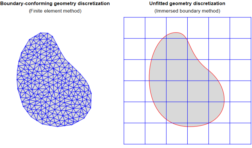
The significance of code verification is especially important when it comes to the research and development of the newest simulation technologies, which are typically based on novel algorithms and often error-prone in-house implementations. Such a numerical framework is the immersed boundary method, where in contrast to the standard FEM , instead of a boundary-conforming geometry discretization, a so-called unfitted discretization is used. An example for these two discretization techniques is depicted below. It is clear that the unfitted mesh, typically based on a Cartesian grid, can be generated with basically no effort. Thus, this simulation technology is well suited for geometries with highly complex boundaries, especially in 3D. As a price for this, advanced algorithms are required that are able to handle the numerical challenges arising in the elements intersected by the domain boundaries (indicated by red color).
In[]:=
Curve=BezierCurve[{{327.0962,55.0152},{455.4455,55.0152},{464.6917,172.1869},{383.8836,234.8131},{315.5726,287.7541},{332.3684,351.9848},{283.8836,351.9848},{179.8432,351.9848},{148.3083,55.0152},{327.0962,55.0152}}];xV=Table[x,{x,xMin,xMax,(xMax-xMin)/6}];yV=Table[y,{y,yMin,yMax,(yMax-yMin)/6}];Lines=Graphics[{Blue,Join[Table[Line[{{x,yMin},{x,yMax}}],{x,xV}],Table[Line[{{xMin,y},{xMax,y}}],{y,yV}]]}];Points=Graphics[{PointSize[0.02],Flatten[Table[Point[{x,y}],{x,xV},{y,yV}],2]}];xMin=120;xMax=520;yMin=0;yMax=400;Grid[{{Text[Style["Boundary-conforming geometry discretization",Bold]],Text[Style["Unfitted geometry discretization",Bold]]},{Text["(Finite element method)"],Text["(Immersed boundary method)"]},{Show[Graphics[{#1,EdgeForm[#2],DiscretizeRegion[DiscretizeGraphics[FilledCurve[Curve],MaxCellMeasure1000]]}],#3,#4],Show[Graphics[{#1,EdgeForm[Red],FilledCurve[Curve]}],Lines,#3,#4]}}]&[LightGray,Blue,ImageSize400,PlotRange{{xMin-5,xMax+5},{yMin-5,yMax+5}}]
1.3 Method of manufactured solution + Immersed boundary methods
1.3 Method of manufactured solution + Immersed boundary methods
Our goal is to utilize the method of manufactured solutions for testing of immersed boundary simulation tools. Note that we use Mathematica solely for the derivation of the manufactured solutions, the numerical simulations themselves are conducted in a different code. A thorough discussion of the typical challenges one is facing in immersed boundary methods is not possible in this post. However, a particular challenge still needs to be mentioned, as it will serve as a basis for all the manufactured solutions discussed below. This challenge is the following: In immersed boundary methods, since no nodes coincide with the boundary, simply assigning prescribed values to a set of boundary nodes like in the FEM is not an option. However, when reproducing a manufactured solutions numerically, all boundaries need to be constrained by boundary conditions, where the constrains take on the field values of the manufactured solution on the boundary.
While it is possible to apply boundary conditions to the immersed boundaries, in our derivations, manufactured solutions are derived for which boundary conditions are readily fulfilled. This can be achieved, e.g., when the manufactured solution results in vanishing normal stresses on the boundary. In this case, homogeneous Neumann boundary conditions are readily fulfilled, and the immersed boundary code can be tested without the need for using advanced constraint algorithms associated with unfitted meshes. Thus, on the one hand, a code verification becomes possible for immersed boundary simulation tools lacking the option of unfitted boundary conditions. On the other hand, the simulation complexity is not increased beyond the necessary level when testing other features of the code.
For more information regarding the given topic, see our open access published papers. From these papers, 3 manufactured solutions are presented below while also indicating in purple which parts correspond to which equations and figures in the papers.
2. Plate witch circular hole – Static analysis
2. Plate witch circular hole – Static analysis
2.1. Governing equations
2.1. Governing equations
In[]:=
LinearStrainTensorPolar[u_]:=Module[{uGrad},uGrad=Grad[u,{r,phi},"Polar"];1/2(uGrad+Transpose[uGrad])]LinearStrainTensor[u_]:=Module[{uGrad},uGrad=Grad[u,{x,y}];1/2(uGrad+Transpose[uGrad])]HookesLawPlaneStress[epsilon_,E_,nu_]:=E/(1-nu^2)*((1-nu)epsilon+nu*Tr[epsilon]*IdentityMatrix[2])BodyLoadStaticPolar[sigma_]:=-Div[sigma,{r,phi},"Polar"]BodyLoadTransientPolar[sigma_,u_,rho_]:=BodyLoadStaticPolar[sigma,u,rho]+rhoD[u,{t,2}]BodyLoadStatic[sigma_]:=-Div[sigma,{x,y}]BodyLoadTransient[sigma_,u_,rho_]:=BodyLoadStatic[sigma]+rhoD[u,{t,2}]StrainEnergyDensity[sigma_,epsilon_]:=1/2(Flatten[sigma].Flatten[epsilon])
2.2. Problem domain definition
2.2. Problem domain definition
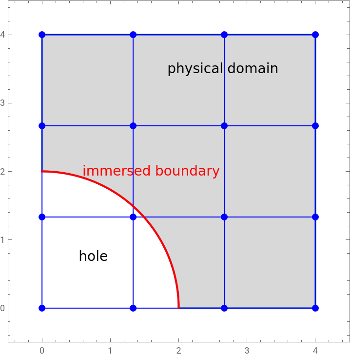
For the first example, a rectangular plate with a circular hole of radius R is investigated. Due to symmetry, only a quarter of the plate is considered. In addition to the physical domain (gray region), also an exemplary unfitted mesh is depicted consisting of 3x3 elements (blue). The red line indicates the boundary piece, where the manufactured solution should result in vanishing tractions.
In[]:=
xMin=0;xMax=4;yMin=0;yMax=4;xC={0,0};R=2;OmegaSquare=ImplicitRegion[x≥xMin&&x≤xMax&&y≥yMin&&y≤yMax,{x,y}];OmegaHole=ImplicitRegion[(x-xC[[1]])^2+(y-xC[[2]])^2≤R^2&&x≥xMin&&x≤xMax&&y≥xMin&&y≤xMax,{x,y}];OmegaPhys=RegionDifference[OmegaSquare,OmegaHole];xV=Table[x,{x,xMin,xMax,xMax/3}];yV=Table[y,{y,yMin,yMax,yMax/3}];Lines=Graphics[{Blue,Join[Table[Line[{{x,yMin},{x,yMax}}],{x,xV}],Table[Line[{{xMin,y},{xMax,y}}],{y,yV}]]}];Points=Graphics[{Blue,PointSize[0.02],Flatten[Table[Point[{x,y}],{x,xV},{y,yV}],2]}];ShowRegionPlot[OmegaPhys,PlotRange->{{xMin-0.5,xMax+0.5},{xMin-0.5,xMax+0.5}},PlotStyleLightGray],Lines,
Out[]=
2.3. Manufactured solution
2.3. Manufactured solution
2.3.1 Define displacement field
2.3.1 Define displacement field
For the current example, the manufactured displacement field is chosen as given below. Note that this definition also contains a parameter c, which will be defined later, such that the displacement field, alongside with chosen material properties, leads to vanishing normal stresses at the hole’s boundary, i.e., for r = R. However, before finding the correct value of c, let the parameter take on various values in the range of c ∈ [0.25, 2.00], resulting in the displacement fields depicted below. Here, the gray area indicates the physical domain (r > R). 〈 Paper [1]: Eq. (28) 〉
In[]:=
u={r*Log[c*r],0};cValues=Table[i,{i,0.25,2,0.25}];Colors=Table[ColorData[3][i],{i,1,Length[cValues]}];ShowTable[Plot[u[[1]]/.{rR,ccValues[[i]]},{R,0,2},PlotStyle{Opacity[0.3],Colors[[i]]}],{i,1,Length[cValues]}],Table[Plot[u[[1]]/.{rR,ccValues[[i]]},{R,2,4},PlotStyle{Colors[[i]]}],{i,1,Length[cValues]}],
2.3.2 Compute strain, stress and body force in polar coordinates
2.3.2 Compute strain, stress and body force in polar coordinates
For the manufactured displacement field, the corresponding strains, stresses and body loads can be easily derived. Below, the Young’s modulus (Emod) and Poisson’s ratio (nu) are used as symbolic variables. 〈 Paper [1]: Eq. (29) 〉
2.3.3 Find value for c, such that the radial stress component is vanishing at the hole’s boundary (r = R)
2.3.3 Find value for c, such that the radial stress component is vanishing at the hole’s boundary (r = R)
Based on the result of the above solution, define a function for c, which, in the current example, only depends on the Poisson’s ratio and radius of the hole. A quick tests reveals that using cRule, the circular boundary is indeed traction-free. 〈 Paper [1]: Eq. (31) 〉
2.3.4 Plotting the radial displacement and stress components
2.3.4 Plotting the radial displacement and stress components
2.4 Strain energy
2.4 Strain energy
Below, a symbolic strain energy density function (SEdens) is derived based on the stress and strain fields resulting from the chosen displacement field. Note that c, Emod, and nu are still symbolic parameters, and r is the radial coordinate. For computing the strain energy, the strain energy density function is integrated over the problem domain, which is realized in two steps: First, the strain energy function is integrated over the entire rectangular domain in Cartesian coordinates. Then, the strain energy in the hole region is computed using radial coordinates. Finally, the actual strain energy is computed by subtracting the previously mentioned two values. 〈 Paper [1]: Eq. (32)–(34) 〉
Finally, an actual value for the strain energy is evaluated using some chosen material parameters. The resulting value is a (i) single scalar solely based on (ii) analytical expressions. Thus, it allows for a simple and reliable reference solution when the same problem is computed numerically via the finite element method, or in case of the published paper: via immersed boundary methods. 〈 Paper [1]: Eq. (32) and Fig. 4b 〉
3. Plate with elliptic inclusion – Transient analysis
3. Plate with elliptic inclusion – Transient analysis
3.1 Problem domain definition
3.1 Problem domain definition
In the second example, a multi-material problem is considered where a matrix material (gray domain) contains elliptic inclusion (orange domain). The inclusion itself is defined by the negative functions values of an implicit level-set function. Additionally, an unfitted mesh containing 2x2 elements is depicted (blue lines). 〈 Paper [1]: Eq. (79) and Fig. 11a 〉
3.2 Key idea for the current manufactured solution
3.2 Key idea for the current manufactured solution
◼
The manufactured problem is formulated in Cartesian coordinates.
◼
In Secs. 3.2.1 and 3.2.2, we first investigate a static manufactured solution for the current problem. Then, in Sec. 3.2.3, the static manufactured solution is turned into a transient one.
3.3 Manufactured solution
3.3 Manufactured solution
3.2.1 Displacement field amplitude
3.2.1 Displacement field amplitude
3.2.2 Derived fields
3.2.2 Derived fields
Using the functions for linear elasticity defined in Sec 2.1, we can easily derive the analytical expression for the strain and stress fields corresponding to the chosen displacement field, as well as the body load field resulting from the stress divergence in the static case. 〈 Paper [1]: Eq. (80) 〉
Plotting the individual field components reveals that while the strains are discontinuous, due to the specific choice of the scaling factor c = Emat/Einc and nuMat = nuInc, all the stress fields are continuous across the material interface. Consequently, the normal stresses are also continuous. Due to the displacement field being a quadratic function resulting from the level-set function, the strains and stresses are linear. Additionally, the body loads, resulting from divergence of the stresses, are constant. It is easy to see that since the stresses are continuous, the body loads are continuous too. 〈 Paper [1]: Fig. 12 〉
3.2.3 Oscillating fields
3.2.3 Oscillating fields
3.4 Reference values for code verification
3.4 Reference values for code verification
For the verification of the numerical simulation, several quantities associated with the manufactured solution can be used. For the chosen example, two comparisons are made.
◼
On the one hand, the x-component of the oscillating displacement field is investigated at the point [0, 0], which is located in the inclusion. The corresponding curve is depicted below on the left for a circular excitation frequency of Ω = 10. 〈 Paper [1]: Figs. 15a and 16a 〉
◼
On the other hand, the global accuracy of the numerical simulation is evaluated by comparing the oscillating strain energy values. The corresponding analytical expression and plot are depicted below. 〈 Paper [1]: Figs. 15b and 16b 〉
4. Plate with cylindrical hole – Nonlinear static analysis
4. Plate with cylindrical hole – Nonlinear static analysis
4.1 Governing equations
4.1 Governing equations
4.2 Problem domain definition
4.2 Problem domain definition
For the current example, a plate with a cylindrical hole is considered. Below, the light blue region depicts the physical domain, and the red surface represents the immersed boundary that is cutting through the elements of the exemplary unfitted mesh. 〈 Paper [2]: Fig. 3a 〉
4.3 Key idea for the current manufactured solution
4.3 Key idea for the current manufactured solution
We have a great freedom in deriving all kinds of manufactured solutions, however, when reproduced numerically via FEM and related techniques, all boundaries must be constrained. While this is not a problem for boundaries which coincide with the nodes, for boundaries located in the interior of the elements (red surface in the above figure), additional steps are needed. Our goal is to derive a manufactured solution, such that tractions on the hole’s boundary are vanishing. Thus, it can be seen as a free boundary, at which homogeneous Neumann boundary conditions are readily fulfilled. This is achieved for the current example due to the following features of the manufactured solution: 〈 Paper [2]: Eqs. (15) and (18) 〉
◼
The cylindrical hole’s outward pointing unit normal vector in a cylindrical coordinate system reads n = [-1, 0, 0].
There are several ways to adjust these parameters, such that the radial stress component vanishes at r = R. For exploring all the possible settings, one may use the built-in Reduce[...] function. In the following, a displacement field is assumed, whose value and first derivative both vanish at the hole’s boundary. The following test reveals that this approach indeed results in zero stresses, regardless of the material properties. 〈 Paper [2]: Eq. (17) and (20) 〉
4.4 Manufactured solution
4.4 Manufactured solution
For the current manufactured solution, a quadratic function is chosen for the radial displacement field component. Some comments regarding the chosen definition for u:
◼
On the one hand, linear problems support the use of more complex functions for the manufactured primary solution field. See, e.g., the logarithmic function that was chosen for the displacement in the first example. On the other hand, non-linear problems are more restrictive in this sense, as for an arbitrary solution field, the derived results can quickly grow out of hand. Since the whole point of using manufactured solutions is to derive reference solutions that can be computed analytically, having a solution field that leads to unsolvable integrals in the end, or expensive symbolic computations, defeats the purpose (see Sec. 4.5).
◼
Note the numerical simulation of non-linear problems is typically conducted using an iterative solution process, e.g., the Newton-Raphson scheme. Thus, we include the so-called load step parameter d ∈ [0,1] into the definition of u, which is then passed on to all the derived quantities, such as the stresses and body loads. In this way, we are able to express the analytical state of system throughout the entire deformation process. 〈 Paper [2]: Eq. (16) 〉
Let us now plot the radial components of the displacement, first Piola-Kirchoff stress, and body load fields for various load step parameters d.. Here, the following observations should be made: 〈 Paper [2]: Fig. 2b 〉
◼
For visualization purposes, the radial displacement component is scaled up by a factor of 100.
◼
For r > 2, the points are located in the physical domain (gray area), while for r < 2, in the hole. The fields not being smooth in the hole does not pose any issues, since we are interested solely in the solution interior to the physical domain.
4.5 Reference values for code verification
4.5 Reference values for code verification
Note that the main goal of the manufactured solution is that one has an analytical reference solution the numerical simulation can be compared to. The comparison can be either local by comparing field values at specific points or global by comparing scalar values that reflect the state of the entire system. Below, we prepare data for a global comparison.
4.5.1 Strain energy
4.5.1 Strain energy
Despite the very simple form of the manufactured displacement field, even this leads to an expression of the strain energy density function that cannot be integrated over the given problem domain analytically. Therefore, the integral value is computed numerically. It is done so for various values of the load step parameter, enabling an insight to how the strain energy of the system grows as the deformation progresses. 〈 Paper [2]: Fig. 4a 〉
CITE THIS NOTEBOOK
CITE THIS NOTEBOOK
Code verification of immersed boundary techniques using the method of manufactured solutions
by Márton Petö, Mahan Gorji, Fabian Duvigneau, Alexander Düster, Daniel Juhre & Sascha Eisenträger
Wolfram Community, STAFF PICKS, May 13, 2024
https://community.wolfram.com/groups/-/m/t/3175245
by Márton Petö, Mahan Gorji, Fabian Duvigneau, Alexander Düster, Daniel Juhre & Sascha Eisenträger
Wolfram Community, STAFF PICKS, May 13, 2024
https://community.wolfram.com/groups/-/m/t/3175245