This study investigates the temporal evolution of the Hubble Space Telescope’s semimajor axis. Information about the Hubble Space Telescope was first obtained using the Wolfram Mathematica knowledge base, which provides direct access to satellite properties and orbital parameters. Using these tools, a time series of the telescope’s semimajor axis was extracted and organized as the primary dataset for the study. The dataset spans 1 January 2020 to 28 February 2026 and was divided into a training set (1 January 2020 to 31 December 2024) and a test set (1 January 2025 to 28 February 2026). To establish a reference for model evaluation, polynomial regression was first used as a baseline model to predict the semimajor axis as a function of time. Although this classical regression approach captures the general orbital trend, its predictive capability remains limited, yielding a coefficient of determination ∼0.46. To improve prediction accuracy, a neural network was then trained on the same dataset. The neural network model demonstrated significantly better performance, achieving a coefficient of determination ∼0.97 on the test dataset. The results indicate that a neural network trained on five years of data can predict the semimajor axis over approximately one year and two months of unseen observations.
2
R
2
R
1 Hubble Space Telescope Overview
1 Hubble Space Telescope Overview
The Hubble Space Telescope is a space-based astronomical observatory launched in 1990 and operating in low Earth orbit. In this section, basic information and orbital parameters of the telescope are retrieved from the Wolfram knowledge base using built-in satellite entities.
Retrieve the list of countries involved in operating the Hubble Space Telescope:
In[]:=
countries=["CountryOfOperatorOwner"]
Out[]=
,,,,,,,,,,,,,,,,,,,,,
Count the total number of participating countries:
In[]:=
Length@countries
Out[]=
22
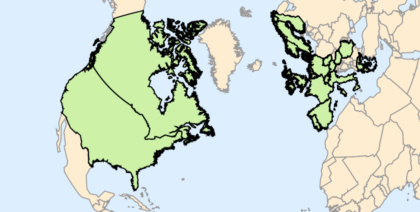
Visualize the geographic distribution of these countries:
In[]:=
GeoGraphics[Style[Polygon[countries],EdgeForm[Black],FaceForm[Green]],GeoBackground"CountryBorders"]
Out[]=
Display key mission information about the Hubble Space Telescope:
In[]:=
GridTranspose,/@,
Out[]=
Name | Hubble Space Telescope |
LaunchDate | |
OrbitType | |
OperatorOwner | {European Space Agency,NASA} |
LaunchSite | Cape Canaveral Air Force Station, Florida, United States |
LaunchMassKg |
Retrieve the current dynamical properties of the telescope:
In[]:=
GridTranspose,/@,
Out[]=
Altitude | |
AverageElevationWGS84 | |
DistanceFromLocation | |
SemimajorAxis | |
AverageVelocity | |
Velocity | |
MeanMotion | |
PeriodOsculating | |
TimeInOrbit |
Extract the current classical orbital elements that determine the telescope’s orbit:
In[]:=
Grid,[#]&/@,
Out[]=
SemimajorAxis | Eccentricity | InclinationOsculating | AscendingNodeLongitude | PerigeeArgument | MeanAnomaly |
0.000172 |
2 Time Series Data Preparation
2 Time Series Data Preparation
In this section, the semimajor axis data of the Hubble Space Telescope from 1 January 2020 to 28 February 2026 is prepared for analysis. The dataset is organized into coordinate pairs, divided into training and test subsets, standardized for numerical stability, and visualized. The standardization step facilitates stable neural network training and reliable prediction.
Generate a daily time sequence from 1 January 2020 to 28 February 2026:
In[]:=
dates=DayRange[{2020,1,1},{2026,2,28}];Short@dates
Out[]//Short=
,,,,2244,,,
Retrieve the semimajor axis data from the Wolfram satellite knowledge base (about 5 minutes; shown for reference):
In[]:=
(*semiMajor=ParallelTableQuantityMagnitude@EntityValue,Dated["SemimajorAxis",date],{date,dates};*)
Access the semimajor axis dataset stored here in compressed form for immediate use:
In[]:=
semiMajor=;Short@semiMajor
Out[]//Short=
{6916.42,6916.42,6916.41,2245,6856.15,6856.1,6856.05}
Combine dates and semimajor axis values into coordinate pairs:
In[]:=
coordinates=Transpose[{dates,semiMajor}];Length@coordinatesShort@coordinates
Out[]=
2251
Out[]//Short=
,6916.42,,6916.42,2248,,6856.05
Define intervals separating the training and test periods:
In[]:=
intervals=Partition[Position[dates,#][[1,1]]&/@{{2020,1,1},{2024,12,31},{2025,1,1},{2026,2,28}},2];Column@intervals
Out[]=
{1,1827} |
{1828,2251} |
Split the dataset into training and test subsets:
In[]:=
{train,test}=coordinates[[#1;;#2]]&@@@intervals;Length/@{train,test}Column[Short[#,2]&/@{train,test}]
Out[]=
{1827,424}
Out[]=
|
|
Convert the dates to numerical values using AbsoluteTime, then Standardize them for numerical stability:
In[]:=
datesSt=N@Standardize[AbsoluteTime/@dates];Short@datesStChop@{Mean[#],StandardDeviation[#]}&@datesSt
Out[]//Short=
{-1.7309,-1.72936,-1.72782,2245,1.72782,1.72936,1.7309}
Out[]=
{0,1.}
Standardize the semimajor axis values:
In[]:=
semiMajorSt=N@Standardize@semiMajor;Short@semiMajorStChop@{Mean[#],StandardDeviation[#]}&@semiMajorSt
Out[]//Short=
{0.888886,0.888839,0.888766,2245,-2.31572,-2.31795,-2.32069}
Out[]=
{0,1.}
Construct standardized coordinate pairs:
In[]:=
coordinatesSt=Transpose[{datesSt,semiMajorSt}];Short@coordinatesSt
Out[]//Short=
{{-1.7309,0.888886},{-1.72936,0.888839},2248,{1.7309,-2.32069}}
Split the standardized dataset into training and test subsets:
In[]:=
{trainSt,testSt}=coordinatesSt[[#1;;#2]]&@@@intervals;Column[Short[#,2]&/@{trainSt,testSt}]
Out[]=
{{-1.7309,0.888886},{-1.72936,0.888839},1823,{1.077,-1.16359},{1.07854,-1.16841}} |
{{1.08008,-1.17258},{1.08162,-1.17783},420,{1.72936,-2.31795},{1.7309,-2.32069}} |
Visualize the original and standardized datasets:
In[]:=
plot=DateListPlot{train,test},;plotSt=ListLinePlot{trainSt,testSt},;Row[{plot,plotSt}," "]
Out[]=


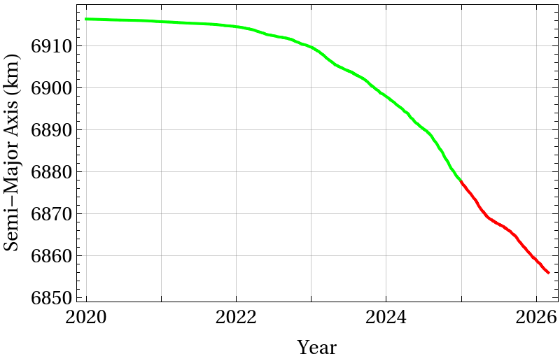
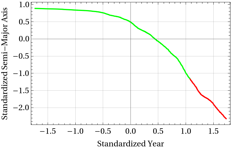
The two panels show the same semimajor axis time series before and after standardization. The left plot presents the original values, while the right plot shows the standardized data used for numerical stability in the modeling process. In the following sections, two predictive models will be constructed: a regularized polynomial regression model and a neural network model. In both cases, the models will be trained using the training set and evaluated on the test set, which consists of previously unseen data.
3 Regularized Polynomial Model Fitting and Selection
3 Regularized Polynomial Model Fitting and Selection
In this section, a family of regularized polynomial regression models is constructed to provide a baseline prediction of the Hubble Space Telescope semimajor axis. Polynomial degrees and regularization strengths were systematically suggested. Fifteen polynomial models were considered, corresponding to degrees from 1 to 15. For each polynomial, seven regularization values were applied, resulting in a total of 105 candidate models. A cost function was then defined based on the root mean square error. This cost was computed for all 105 models using both the training and validation datasets. The resulting cost values were visualized using MatrixPlot, where colors represent the magnitude of the loss values, allowing the most suitable model to be identified easily through visual inspection. After selecting the optimal configuration, the chosen model was further evaluated using additional performance measures. The overall procedure of proposing candidate models and selecting the most suitable one follows the standard model selection framework described in the book Introduction to Machine Learning by Etienne Bernard.
Prepare the regression dataset by converting dates to numerical time values and split the training data into fitting and validation subsets:
Construct polynomial basis functions of increasing degree to generate candidate model structures with different levels of complexity:
Define the set of regularization hyperparameters used in the Tikhonov regularization experiments:
Fit regularized polynomial regression models for all combinations of polynomial degree and regularization strength:
Generate model predictions for the full dataset and separate the predicted values into training and validation segments:
Define a cost function based on RootMeanSquare error and compute the training and validation costs for all model configurations:
Visualize the cost matrices to identify the optimal combination of polynomial degree and regularization strength:
The training cost matrix indicates that the third-degree polynomial yields the lowest cost, with negligible differences among its regularization values. In the validation matrix, the fourth-degree polynomial achieves the lowest cost with similarly minor variation across regularization values. Therefore, the fourth-degree polynomial with the first regularization value is selected as the final model.
Select the polynomial model corresponding to the lowest validation cost identified in the MatrixPlot:
Evaluate the selected polynomial model over the complete time range to obtain predicted semimajor axis values:
Construct coordinate pairs of dates and fitted semimajor axis values:
Separate the fitted data into training, validation, and test subsets:
Overlay the fitted curves with the original observations to visualize model performance:
Compute the residuals between observed and fitted semimajor axis values:
Extract the residuals corresponding to the test dataset:
Compute the standard deviation of the test observations:
4 Neural Network Regression Model
4 Neural Network Regression Model
In this section, an alternative modeling approach based on neural networks is developed in an attempt to obtain improved predictive performance compared with the polynomial regression model. A neural network is constructed and trained using the standardized time series data of the semimajor axis. During training, regularization techniques are applied to control model complexity and reduce the risk of overfitting, following the guidelines described in the Wolfram Documentation Center (Training Neural Networks with Regularization). The evaluation and analysis of the trained model are then carried out using standard predictive performance measures and diagnostic tools, following the model assessment principles discussed in the book Introduction to Machine Learning by Etienne Bernard.
Train the neural network using the standardized training data with stochastic gradient descent and L2 regularization:
Extract the trained neural network to construct the prediction function:
Evaluate the trained network over the standardized time inputs and rescale the predictions to the original semimajor axis units:
Construct coordinate pairs of dates and neural network predictions:
Separate the predicted values into training and test segments:
Overlay the neural network predictions with the original observations to visualize model performance:
The neural network predictor closely follows the observed semimajor axis evolution across both the training and test intervals. Compared with the polynomial curve fitting model, the neural network provides a noticeably more accurate approximation of the data.
Compute the residuals between observed and predicted semimajor axis values:
Extract the residuals corresponding to the test dataset:
Visualize the test residuals over time to examine prediction errors:
Visualize the distribution of residuals and compare it with the distribution of the test observations:
The residual histogram shows that most prediction errors are concentrated near zero, indicating that the model does not exhibit a strong systematic bias toward over- or under-prediction. Only a small number of observations appear in the outer bins, suggesting that large outliers are limited. The histogram of the test set is shown alongside the residual histogram to provide a reference scale, illustrating that the magnitude of the prediction errors is small compared with the overall range of the semimajor axis values.
Summarize the prediction errors using absolute and relative error statistics:
Compute the standard deviation of the test observations (used in subsequent calculations):
Create a comparison plot of predicted and actual values to assess prediction accuracy relative to perfect predictions:
Identify the largest and smallest prediction errors along with their corresponding dates, predicted values, and actual values:
Display structural information about the trained neural network:
Retrieve the list of available neural network properties:
Display the explicit input-form representation of the trained neural network:
Report the number of each layer type in the network architecture:
Display a graphical summary of the neural network architecture:
Display the internal MXNet computational graph of the neural network:
Retrieve the available predictor properties of the trained model:
Display the full training network, including the loss function:
Report the total training time, number of training rounds, processed batches, and batch size:
Display the optimization configuration used during training:
Display the training and validation loss curves recorded during the optimization process:
This study treats the semimajor axis primarily as a time series dataset and focuses on predictive modeling rather than on the physical interpretation of orbital evolution. In particular, the analysis does not attempt to determine the physical causes of the observed decrease in the semimajor axis, which might be associated with atmospheric drag in low Earth orbit or with a combination of perturbing forces. Moreover, the origin of the irregular variations in the decay trend is not known. It is unclear whether these fluctuations arise from observational inaccuracies or from physical perturbations acting on the orbit. Determining the source of this behavior is important for model construction, since the appropriate modeling approach depends on whether the variability reflects measurement noise or genuine dynamical effects. These questions remain open and provide promising directions for future research. One possible extension would be the development of models capable of learning and interpreting the influence of perturbations by comparing ideal two-body orbital motion with both fully perturbed dynamical models and observational datasets. Such comparisons may help reveal the underlying structure and relative behavior of the perturbing forces that shape the evolution of satellite orbits.
Resources
Resources
◼
◼
◼