Abstract
Abstract
Swarm robotics refers to the study of collective behaviour that emerges from collaboration between multiple simple robots. Swarm robotic systems are frequently used in area-exploration and environment-mapping tasks. This project proposes graph-theory based approaches for the multi-robot exploration of enclosed spaces with both known and unknown boundaries. Simulations of these approaches on swarms of up-to ten robots were run and they were able to explore 100% of the enclosed space with a higher rate of area-exploration than random walk methods.
Introduction
Introduction
Problem Statement and Motivation
Problem Statement and Motivation
The aim of this project is to find an optimized method for exploring an enclosed space using a swarm of multiple simple robots. Area-exploration is an important application of swarm robotic systems. These systems can be used to identify survivors in dangerous environments, for instance, during search and rescue operations in fire-ground environments. They may also be used to map large environments, vacuum clean an enclosed space or even for planetary exploration. The methods proposed in this project would increase the efficiency of the aforementioned tasks and maximize area explored.
The following assumptions about the swarm robotic system and enclosed space will be made in this project:
The following assumptions about the swarm robotic system and enclosed space will be made in this project:
◼
The enclosed space is assumed to be a convex polygon, and robots are randomly placed within the enclosed space.
◼
Robots are small-sized relative to the size of the enclosed space and move with the same constant speed.
◼
The starting positions of all robots are known and, at any given point in time, robots are able to determine their positions relative to their starting position.
◼
Since a swarm robotic system is being considered, robots are able to communicate and share data with one another.
◼
Robots are only able to sense obstructions in the enclosed space that are directly in-front of them.
◼
No objects, apart from the robots, are placed in the enclosed space. Hence, the only obstructions present in the environment for a given robot are other robots and the walls of the enclosed space.
Since the area of the enclosed space and the number of robots in the swarm have not been specified, the methods proposed must work for all sizes of enclosed spaces and any number of swarm robots. Furthermore, the time taken to compute the paths of the robots can also be considered negligible in comparison to the time taken for the process of area-exploration.
Since the area of the enclosed space and the number of robots in the swarm have not been specified, the methods proposed must work for all sizes of enclosed spaces and any number of swarm robots. Furthermore, the time taken to compute the paths of the robots can also be considered negligible in comparison to the time taken for the process of area-exploration.
Approach to Problem
Approach to Problem
The enclosed space will be considered a discrete space in this project. Robots will be initially placed at random lattice points (points with integer coordinates) and will only be able to move between lattice points that lie within the enclosed space. A discrete space would make it easier to measure the area explored by the robot, which can be measured as the percentage of lattice points visited by the robot.
Since the most simple approach to exploring an enclosed space would be a random walk, this project uses a random walk method as a benchmark for comparing other approaches. After considering random walks, this project proposes methods for two separate cases of the problem–the boundaries of the enclosed space are known and the boundaries of the enclosed space are unknown. Knowledge of the boundaries of the enclosed space could inform and significantly optimize path-planning. Certain swarm robotic systems, such as vacuum cleaning robots, may have information about the shape and size of the enclosed space, while others, such as search and rescue robots, may not. Thus, these cases were considered separately.
Generating the Enclosed Space
Generating the Enclosed Space
As mentioned previously, the enclosed space is assumed to be an enclosed polygon. In order to generate a random convex polygon, we can first assume a random circle of a specified size and select points that lie on the circle to represent vertices of the convex polygon. Since all vertices of the polygon are the same distance away from the centre of the circle, the polygon generated will always be convex.
Function to create a list of vertices for a convex polygon:
In[]:=
convexPolygon[size_,vertices_]:=(AngleVector[{size,#}]&/@Sort[RandomReal[{-Pi,Pi},vertices]])
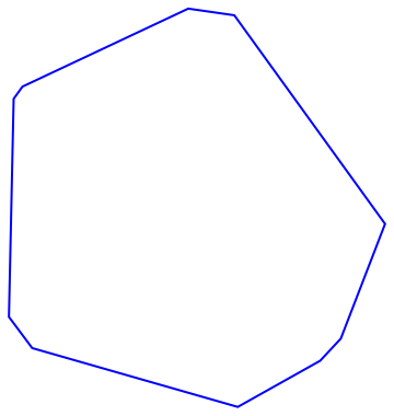
Generate a convex decagon of size 20 units:
In[]:=
spaceVertices=convexPolygon[20,10];space=Polygon[spaceVertices];Graphics[{FaceForm[],EdgeForm[Blue],space},ImageSizeSmall]
Out[]=
Calculating the approximate bounds of the polygon:
In[]:=
polygonBounds=Table[{Floor[Min[spaceVertices]],Ceiling[Max[spaceVertices]]},2];
Point in Polygon
Point in Polygon
Since robots can not leave the enclosed space, approaches proposed in this project would need a method to determine whether or not a given point lies within the enclosed space. Such a method would be analogous to sensors on the robot which would allow it to sense the walls of the enclosed space and determine whether or not the point directly in-front of it lies within the enclosed space.
Function to determine whether or not a given point lies within the polygon defined by the given list of vertices:
In[]:=
pointInPolygon[pt_,polygonVertices_]:=(CrossingCount[Line[Join[polygonVertices,{polygonVertices[[1]]}]],pt]==1)
Bounded Random Walk
Bounded Random Walk
A random walk consists of a series of randomly selected steps. In a bounded random walk, the random walk is not allowed to cross a certain boundary, in this case, the boundary of the enclosed space.
Although the methods proposed in this project would work for any number of robots in the system, for demonstration purposes, a swarm robotic system with four robots is considered.
Although the methods proposed in this project would work for any number of robots in the system, for demonstration purposes, a swarm robotic system with four robots is considered.
Number of robots in the swarm robotic system:
In[]:=
robotCount=4;
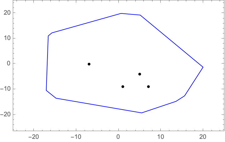
Since the robots are assumed to be randomly placed in the environment, we can generate a list of four random points within the enclosed space to represent the start positions of the robots.
In[]:=
generatePointInPolygon[size_,polygonVertices_]:=If[pointInPolygon[#,polygonVertices],#,generatePointInPolygon[size,polygonVertices]]&@RandomInteger[{-size,size},2]
Generating robot start positions:
In[]:=
robotStartPositions=Table[generatePointInPolygon[10,spaceVertices],robotCount];
Displaying robot start positions in the enclosed space:
In[]:=
robotStartPositionsPlot=ListPlot[robotStartPositions,PlotStyle->Black];ShowrobotStartPositionsPlot,Graphics[{FaceForm[],EdgeForm[Blue],space}],
Out[]=
During the random walk, each robot will take a random step in one of four directions–left, right, forwards or backwards:
In[]:=
directionList={{1,0},{0,1},{-1,0},{0,-1}};randomDirection:=RandomChoice[directionList];
Function which takes a random step from the given point, ensuring that the step lies within the enclosed space:
In[]:=
randomStep[pt_,polygonVertices_]:=If[pointInPolygon[#,polygonVertices],#,randomStep[pt,polygonVertices]]&@(pt+randomDirection)
Function which performs a random step from each of the points in the list of points:
In[]:=
randomWalk[pts_,polygonVertices_]:=randomStep[#,polygonVertices]&/@pts
Each robot performs a bounded random walk of 500 steps from its start position:
In[]:=
randomWalkList=Block[{$IterationLimit=5000},Transpose@NestList[randomWalk[#,spaceVertices]&,robotStartPositions,500]];
ShowListLinePlot[randomWalkList],Graphics[{FaceForm[],EdgeForm[Black],space}],robotStartPositionsPlot,
Out[]=
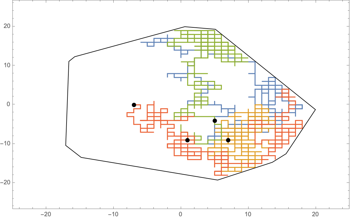
Bounded random walks are quite inefficient at area exploration. This is primarily due to the fact that robots’ paths overlap. There may also be collisions between robots in larger swarms.
Space Partitioning
Space Partitioning
In order to prevent overlaps between robot paths, the enclosed space could be partitioned into sub-regions, with each robot exploring the sub-region that they are in. Each sub-region should contain exactly one robot. A Voronoi Diagram has been considered for space partitioning.
Voronoi Diagram
Voronoi Diagram
Compute the Voronoi Diagram based on the initial positions of the robots:
In[]:=
region=DiscretizeGraphics@space;voronoiDiagram=VoronoiMesh[robotStartPositions,polygonBounds];
Enclosed space and the Voronoi Diagram:
In[]:=
Row[{region,voronoiDiagram}]
Out[]=
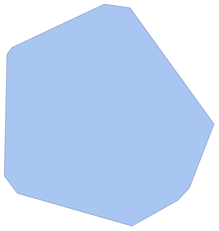
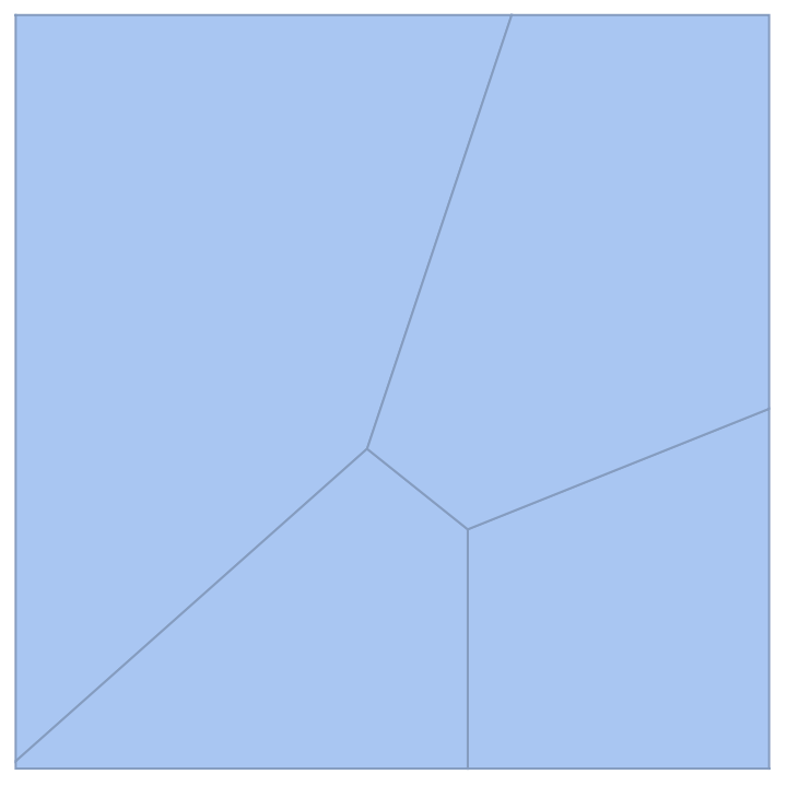
In order to generate the sub-regions for each robot, the intersections of the enclosed space and the Voronoi Diagram will have to be computed.
In[]:=
subRegions=RegionIntersection[DiscretizeGraphics@#,region]&/@MeshPrimitives[voronoiDiagram,2];subPolygonVertices=MeshCoordinates/@subRegions;
Ensuring that robotStartPositions are ordered such that each robot starts within the sub-region at the corresponding index in subRegions:
In[]:=
robotStartPositions=Table[SelectFirst[robotStartPositions,pointInPolygon[#,subPolygonVertices[[i]]]&],{i,robotCount}];
Improved Random Walk
Improved Random Walk
We can perform an improved bounded random walk using the sub-regions generated by the Voronoi Diagram.
Function for random walks in the generated sub-regions:
Each robot performs a bounded random walk of 500 steps from its start position, within its sub-region:
This is certainly an improvement, as robots’ paths overlap less and collisions are not possible, because each robot is restricted to its subregion. However, this approach is still quite inefficient.
Exploration of a Known Enclosed Space
Exploration of a Known Enclosed Space
As previously mentioned, two cases of area exploration are considered–the enclosed space boundaries are known, the enclosed space boundaries are unknown. This section deals with the first case, that is, the exploration of a known enclosed space. If the boundaries of the enclosed space are known, all lattice points that lie within the enclosed space can be computed. Robots could also move between points that are farther than one unit apart, since they know that there are no walls between them.
An graph theory based approach to the known enclosed space case has been considered. All the lattice points in a given sub-region are treated as nodes of an undirected graph, in which weights of any edge between two nodes (lattice points) is equal to the Euclidean distance between them. A shortest tour of this graph, starting at the initial position of the robot, would be the most efficient method of exploring the enclosed space with known boundaries.
Lattice Points inside Enclosed Space
Lattice Points inside Enclosed Space
In order to compute lattice points within each sub-region of the enclosed space, a list of all lattice points within the bounds of the enclosed region are computed and any points that do not lie within the given sub-region are removed from the list.
Computing lattice points within each sub-region:
Moving the robot start positions to the front of the list of lattice points:
Shortest Tour
Shortest Tour
A Hamiltonian Cycle is a graph cycle that passes through all nodes in the graph exactly once. The FindShortestTour function finds the shortest Hamiltonian Cycle starting at the starting position of the robot, which visits all nodes (lattice points), in the robot’s sub-region. This is the shortest path visiting all lattice points in the sub-region that ends at the starting position of the robot. The FindShortestTour function has several options for the method that it uses to compute the shortest tour.
List of available methods for the FindShortestTour function:
Computing robot paths for all methods in methodsList:
Select colors for the path of each robot:
Displaying computed robot paths for all methods in methodsList:
The “Automatic” method of FindShortestTour resulted in the minimum total distance travelled by all robots. Thus, the “Automatic” method of FindShortestTour will be used in order to compute robot paths.
Optimization using Lloyd’s Method
Optimization using Lloyd’s Method
Area-exploration in the known enclosed space case can be further optimized using Lloyd’s Relaxation Algorithm. In the Voronoi Diagram shown previously, due to the arrangement of the initial positions of the robots, areas of computed sub-regions may be significantly different from one another. This is sub-optimal because if, for instance, one sub-region is much smaller than the others, the robot in that sub-region would be able to explore the sub-region much faster than other robots and would have to sit idle until the other robots finished their exploration tasks. The time taken by the area-exploration process is determined by the robot that takes the longest time to navigate its sub-region. Thus, in order to make the process even more efficient, areas of sub-regions should be as close to each other as possible.
Lloyd’s Method can be used to compute evenly spaced points within a specified region, which can be partitioned into almost equally sized convex sub-regions. Lloyd’s algorithm is an iterative method that can be performed on a set of starting points. The method is summarised by the steps below:
1
.Compute the Voronoi Diagram for the given list of points
2
.Identify the centroids of each sub-region of the Voronoi Diagram
3
.Move each given point to the centroid of its Voronoi Diagram sub-region
The method can then be re-performed on the list of points obtained in step 3. After multiple iterations of this algorithm, the points become evenly spaced, and the areas of sub-regions in the Voronoi Diagram become approximately equal.
A resource function will be to perform Lloyd’s method. The function accepts a region, a set of starting points and the number of iterations as inputs, and performs the specified number of iterations of Lloyd’s method on the set of points. The sub-regions computed by this resource function depend on the region inputted. In this case, the region representing the enclosed space will be passed in.
Lloyd’s Method resource function:
Running 100 iterations of Lloyd’s Method on robot starting positions and rounding the results to the nearest lattice points:
The points are more spaced out after running Lloyd’s Method:
Voronoi Diagram after performing Lloyd’s Method:
Areas of sub-regions are closer to each other after performing Lloyd’s Method:
Computing sub-regions generated from the updated Voronoi Diagram:
Ensuring that lloydStartPositions are ordered such that each robot starts within the sub-region at the corresponding index in lloydSubRegions:
Computing lattice points within each updated sub-region:
Computing new robot paths for all methods in methodsList:
The areas of sub-regions explored by each robot are almost equal. Thus, finding the shortest tour of each sub-region computed after Lloyd’s Method is an optimized approach of area exploration when boundaries of the enclosed space are known.
Exploration of an Unknown Enclosed Space
Exploration of an Unknown Enclosed Space
This section deals with the second case, that is, the exploration of an unknown enclosed space. Since the boundaries of the enclosed space are unknown, robots can no longer travel between lattice points that are further than one unit apart. This is because robots are not aware of whether or not there are walls between those two points. Robots can only travel one unit at a time because of the assumption that they can only sense obstacles or walls directly ahead of them. Since there is insufficient information about the enclosed space, a graph can not be constructed, hence shortest tours can not be found using the FindShortestTour function.
However, at any given point, the robot has knowledge of whether or not it can move to lattice points to the left, right, front or back of it. If every lattice point is considered a node in the graph, nodes adjacent (connected) to that node can be determined. Thus, a modified depth-first-search can be implemented which only requires information of the adjacent nodes to the node that the robot is currently at.
Since Voronoi Diagrams can be computed using information about the starting positions of robots only, the modified depth-first-search will be performed by each robot within its sub-region determined by the Voronoi Diagram.
Modified Depth-First-Search
Modified Depth-First-Search
Function to get all adjacent lattice points to a given point, that lie within the enclosed space:
Modified depth-first-search (DFS):
Computing robot paths using the modified DFS function:
Displaying the computed robot paths:
Since Lloyd’s method requires information about the region (enclosed space) in which robots are spaced, it can not be used to optimize the modified depth-first-search approach. Nevertheless, if some information about the enclosed space is known (for example, its size or bounds), then it can be approximated by a rectangle or circle. In that case, Lloyd’s method could still be used to optimize the modified depth-first-search approach.
Simulations and Results
Simulations and Results
In order to quantitatively determine which area-exploration approach is most efficient, simulations were performed. In each simulation, the enclosed space was kept the same: a 15 sided convex polygon with size 25 units. The following area exploration methods were considered:
1
.Bounded Random Walk
2
.Bounded Random Walk within Voronoi Diagram sub-regions
3
.FindShortestTour within Voronoi Diagram sub-regions
4
.Modified Depth-First-Search within Voronoi Diagram sub-regions
5
.FindShortestTour within Voronoi Diagram sub-regions (optimized by Lloyd’s Method)
Each of the aforementioned methods were tested in swarm robotic systems of size 1, 2, 4, 6, 8 and 10 robots. Robot paths for each method-robot count configuration were recorded and evaluated based on the following metrics:
◼
Area Explored - This was measured as the percentage of lattice points within the enclosed space that were visited by the robot swarm.
◼
Time Taken for Area-Exploration - Since all robots travel at the same constant speed, the robot that takes the longest time for traversing its path would determine how long the entire system takes. Thus, the time taken for area-exploration by the system can be approximated by taking the length of the longest path travelled by any robot in the swarm system.
◼
Rate of Area Exploration - This was measured by dividing “Area Explored” by the “Time Taken for Area-Exploration”
Simulation Robot Paths
Simulation Robot Paths
The following section contains plots of robot paths for all of the simulations run.
Generating all of the line plots for robot paths:
Grid showing robot paths for all method-robot count configurations:
Simulation Data Plots
Simulation Data Plots
The lattice points of the simulated enclosed space:
Calculating area explored in each simulation, for all of the aforementioned methods:
Calculating time taken by the robots in each simulation, for all of the aforementioned methods:
Calculating the rate of area exploration by robots in each simulation, for all of the aforementioned methods:
Plotting processed simulation data:
Simulation Data Analysis
Simulation Data Analysis
Based on the “Proportion of Area Explored” plot, we can see that Methods 3, 4, 5 are able to explore ~100% of the enclosed space for all sizes of robot swarms simulated. Methods 1 and 2 (random walk based methods), however, were not able to explore more than 40% of the area in each simulation.
The “Time Taken for Area Exploration” plot indicates that, while Methods 1, 2, 3 and 5 take a similar duration of time for area exploration, Method 4 takes a significantly longer duration of time in each case. This can be attributed to the inefficient nature of the exhaustive depth-first-search process. We can see a drastic reduction in time taken from Method 4 to Method 5, which indicates that information about the boundaries of the enclosed space can significantly improve the efficiency of the area-exploration approach.
With reference to the “Rate of Area Exploration” plot, we can see that Method 5 has a significantly greater rate of exploration than Method 3, which suggests that Lloyd’s Method has significantly optimized the area-exploration process. Method 5 has the greatest rate of area exploration, thus, it is the most efficient method for known-space area-exploration. While Method 4 has a low rate of area exploration, it is able to consistently explore 100% of the enclosed space. Thus, Method 4 would be the preferred method of area-exploration for the unknown-space case.
Another interesting observation that can be made from the “Rate of Area Exploration” plot is that the rate of area-exploration increases as the number of robots in the swarm increases. This supports the statement that swarm robotic systems with multiple robots are particularly useful for area exploration.
Conclusion
Conclusion
In conclusion, FindShortestTour within Voronoi Diagram sub-regions (optimized by Lloyd’s Method), or Method 5, was the most efficient method for area-exploration for an enclosed space with known boundaries. It was able to consistently explore 100% of the enclosed space across all sizes of robot swarms simulated. Furthermore, it was 2.00 times more efficient at area exploration than FindShortestTour within Voronoi Diagram sub-regions (without Lloyd’s Method), which indicates that Lloyd’s Method significantly increased the rate of area-exploration. For the unknown enclosed space case, the Modified Depth-First-Search within Voronoi Diagram sub-regions, or Method 4, is the preferred method of area-exploration. Despite the fact that this method had a lower rate of area-exploration than random walk methods (Methods 1, 2), it is able to consistently explore 100% of the enclosed space. Since area-exploration has been prioritized over efficiency, the Modified Depth First Search is preferred over random walks for the unknown enclosed space case.
I believe that this project has achieved its aim of finding an optimized method for exploring an enclosed space using a swarm of multiple simple robots.
Further Steps
Further Steps
This project makes assumptions about the enclosed space in order to simplify the task of finding an optimized area exploration method. In the future, these assumptions can be addressed in order to create an even more efficient and versatile approach. In future projects, non-convex enclosed spaces could also be considered. This would make it more challenging to construct Voronoi Diagrams. Thus, new space partitioning methods could also be investigated. An important improvement that could be made to this project would be to consider obstacles or obstructions present in the enclosed space, to better represent a real life situation. In order to improve the efficiency of the existing method for unknown enclosed space area-exploration, non-exhaustive exploration methods could also be considered, for example, the use of discrete spirals or other space filling curves, which could be designed to consistently explore a certain percentage of the area of the enclosed space. Lastly, a continuous space could also be considered, where robots are not restricted to moving between lattice points.
Acknowledgements
Acknowledgements
I would like to thank my mentor, Zach Shelton, for his guidance and support throughout the course of this project. I am grateful for being given the opportunity to discuss my work with Dr. Stephen Wolfram and Christopher Wolfram. I would also like to thank all of the TAs, mentors and staff members at the Wolfram Summer Camp 2021 for their help and efforts to make camp an extremely interesting and enjoyable experience.
References
References
◼
Voronoi Diagram. (2021). Wolfram.com; Wolfram Research, Inc. https://mathworld.wolfram.com/VoronoiDiagram.html
◼
LloydAlgorithm | Wolfram Function Repository. (2020). Wolframcloud.com; Wolfram Function Repository. https://resources.wolframcloud.com/FunctionRepository/resources/LloydAlgorithm/
◼
Traveling Salesman Problem - Wolfram Demonstrations Project. (2011). Wolfram.com. https://demonstrations.wolfram.com/TravelingSalesmanProblem/
◼
Depth First Search or DFS for a Graph - GeeksforGeeks. (2012, March 15). GeeksforGeeks. https://www.geeksforgeeks.org/depth-first-search-or-dfs-for-a-graph/
◼
Alhalabi, W., Kitanneh, O., Alharbi, A., Balfakih, Z., & Sarirete, A. (2016). Efficient solution for finding Hamilton cycles in undirected graphs. SpringerPlus, 5(1). https://doi.org/10.1186/s40064-016-2746-8
Keywords
Keywords
◼
Random Walk
◼
Voronoi Diagram
◼
Hamiltonian Cycle
◼
Depth-First-Search (DFS)
◼
Lloyd’s Algorithm