The Nusselt Problem
Authors: Housam Binous and Ahmed Bellagi
The Nusselt Problem
Authors: Housam Binous and Ahmed Bellagi
Authors: Housam Binous and Ahmed Bellagi
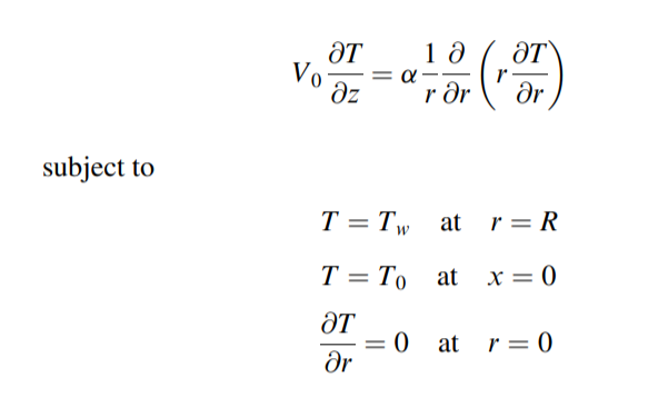
We consider the problem of heat transfer in plug flow heat exchanger .
This problem is similar to the Graetz problem where the velocity profile is laminar .
Axial conduction is ignored .
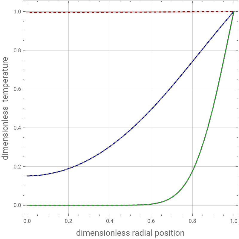
We determine the temperature profile obtained using NDSolve at different local residence times .
We also provide a solution based on orthogonal collocation.
Description of the orthogonal collocation method using Chebyshev-Gauss-Lobatto points is given in the following paper:
H. Binous, A. Shaikh and A. Bellagi, Chebyshev Orthogonal Collocation Technique to Solve Transport Phenomena Problems With Matlab and Mathematica, Computer Applications in Engineering Education, 23(3), pp. 422–431, 2015.
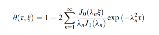
We show that the analytical solution (derived in details in Ref. 1) gives the same result as their counterparts obtained using NDSolve and orthogonal collocation.
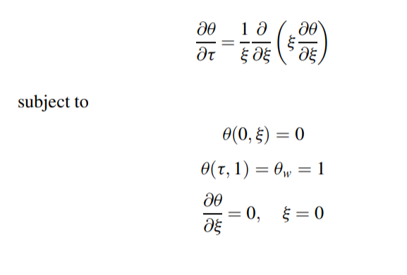
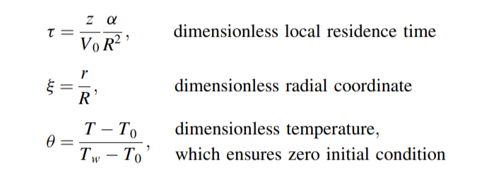
Acknowledgement :Governing equations and analytical solution of the Nusselt problem are reproduced from Ref. 1.In dimensionless form, the problem reduces to :whereReferences:1- Rice and Do, Applied Mathematics and Modeling for Chemical Engineers, 2nd Ed. , New-York: Wiley, 2012, pp. 252-253.
In[]:=
Off[General::"spell1"]
Solution using NDSolve
In[]:=
sol=NDSolveD[θ[τ,ξ],{τ,1}]D[ξD[θ[τ,ξ],{ξ,1}],{ξ,1}],θ[0,ξ]Exp[-1000(1-ξ)],θ[τ,1]1,(D[θ[τ,ξ],{ξ,1}]/.ξ10^-8)0,{θ[τ,ξ]},{τ,0,10},{ξ,10^-8,1}
1
ξ
Out[]=
θ[τ,ξ]InterpolatingFunction[τ,ξ]


In[]:=
plt=Plot[{First[θ[τ,ξ]/.sol]/.τ->1,First[θ[τ,ξ]/.sol]/.τ->0.1,First[θ[τ,ξ]/.sol]/.τ->0.01},{ξ,10^-8,1},PlotRangeAll,PlotStyle{Darker@Red,Darker@Blue,Darker@Green},Frame->True,GridLines->Automatic,FrameLabel->{Style["dimensionless radial position",14],Style["dimensionless temperature",14]},ImageSize->400{1,1},AspectRatio->1,PlotLegends->{Style["τ=1",14,Darker@Red],Style["τ=0.1",14,Darker@Blue],Style["τ=0.01",14,Darker@Green]}];
In[]:=
Show[plt]
Out[]=
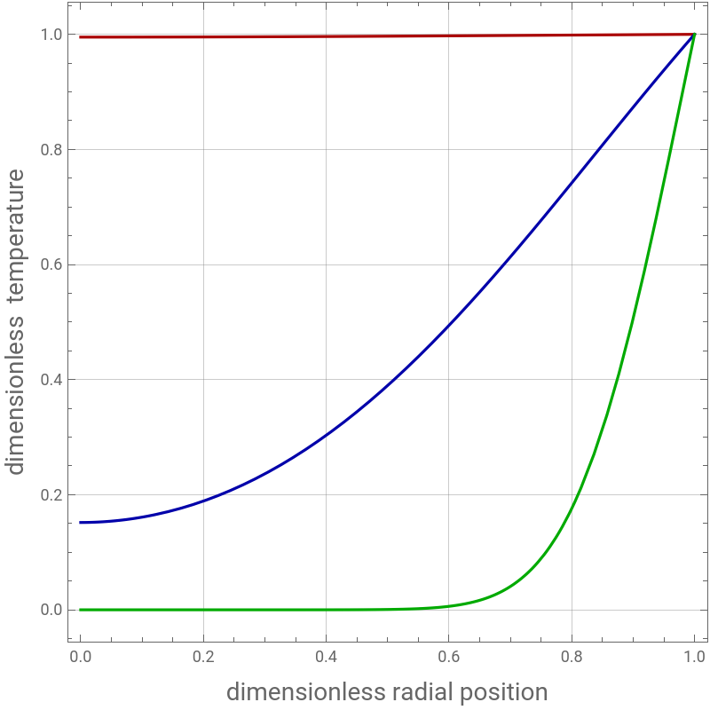


Analytical Solution gives same result as the one obtained using NDSolve

In[]:=
n=1;
In[]:=
While[n<10,{=FindRoot[BesselJ[0,x]0,{x,nPi}][[1,2]],Print[],n++}]
λ
n
λ
n
2.40483
5.52008
8.65373
11.7915
14.9309
18.0711
21.2116
24.3525
27.4935
In[]:=
θanal[τ_,ξ_]:=1-2BesselJ[1,]Exp[-^2τ]
9
∑
n=1
BesselJ[0,ξ]
λ
n
λ
n
λ
n
λ
n
In[]:=
τ=1;
In[]:=
plt4=Quiet@Plot[First[θanal[τ,ξ]/.sol],{ξ,10^-8,1},PlotRangeAll,PlotStyle{Dashed,LightGray,Thick}];
In[]:=
τ=0.1;
In[]:=
plt5=Plot[First[θanal[τ,ξ]/.sol],{ξ,10^-8,1},PlotRangeAll,PlotStyle->{Dashed,Gray,Thick}];
In[]:=
τ=0.01;
In[]:=
plt6=Plot[First[θanal[τ,ξ]/.sol],{ξ,10^-8,1},PlotRangeAll,PlotStyle{Dashed,Gray,Thick}];
Comparison results with NDSolve and analytical solution
In[]:=
Show[plt,plt4,plt5,plt6]
Out[]=
Solution using orthogonal Collocation and Chebyshev-Gauss-Lobatto points
Comparison results with NDSolve (solid lines) and orthogonal collocation solution (dots)