Portfolio optimization is a fundamental financial concept that appears straightforward in theory, yet the practical implementation of efficient diversification strategies presents significant computational and coordination challenges. However, with deeper analysis, the construction of optimal portfolios using mean-variance optimization reveals complex mathematical relationships between risk and return that, when modeled through efficient frontier analysis, leads to sophisticated investment strategies with realistic market applications. In this project, portfolio optimization is modeled using the mean-variance framework through historical stock data analysis, calculating weighted average returns and covariance matrices to estimate expected returns and assess inter-asset relationships. These calculations are then integrated into a decentralized framework that enables distributed portfolio decision-making without reliance on central authority, focusing on two key portfolio types: the minimum variance portfolio and the naturally efficient portfolio positioned along the efficient frontier. This approach is applicable to real-world scenarios such as institutional asset management and autonomous trading systems. In addition, the same decentralized logic can be extended to model other applications in financial technology such as algorithmic trading networks and distributed investment platforms.
1. Introduction
1. Introduction
This paper presents a decentralized approach to optimizing stock portfolios using the concept of the mean variance frontier. Beginning with the collection of historical stock data, the study calculates the weighted average returns to estimate expected returns. Covariance matrices are then derived to estimate expected returns. Covariances matrices are then derived to access relationship between assets. These inputs are then used to model the 2 key portfolio types the minimum variance & naturally efficient portfolio which are positioned along the efficient frontier. The program integrates these calculations into a decentralized framework that allows for distributed portfolio decision making without a reliance on a central authority.
2. The Mean Variance Frontier
2. The Mean Variance Frontier
The Mean Variance Frontier Equation calculates the total risk (variance) of a portfolio made by combining two other portfolios. It accounts for the individual risks of each component and how they move together (their correlation). By adjusting the weight between the two, it helps determine how risk behaves as the mix changes. This analysis is motivated by the need to identify optimal portfolio allocations that maximize expected returns for given risk levels, enabling investors to make informed decisions about risk-return trade-offs.
2
σ
2
W
p
2
σ
*
w
p
2
σ
mv
W
p
W
p
r
*
r
mv
3. Financial Analysis
3. Financial Analysis
3.1 Global Variables
3.1 Global Variables
As an initial case study for this paper, we will consider an investment in three stocks over a specific time period. This simplified three-asset framework provides a manageable yet meaningful demonstration of portfolio optimization principles, allowing for clear visualization of diversification benefits and risk-return relationships without the complexity of larger portfolios.
In[]:=
stockList={"GOOG","AAPL","IBM"};startDate={2020,1,1};endDate={2022,12,31};dates={startDate,endDate};
3.2 Data Retrieval
3.2 Data Retrieval
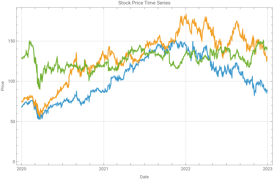
The FinancialData function retrieves all the required data for the respective dates & stock the user mentioned and then provides a visual demonstration of the stock trajectory over that time frame. This approach enables users to quickly grasp market trends, identify patterns in price movements, and make more informed investment decisions by presenting complex financial data in an intuitive, easy-to-understand visual format rather than overwhelming them with raw numerical data.
In[]:=
holdDays=252;
This retrieves all the financial data over the period of time requested by the user ( specific in the stockList & dates variable ).
In[]:=
timeSeries=FinancialData[#,dates]&/@stockList;
Visualizes the financial data over a graph
In[]:=
DateListPlot[timeSeries,PlotLegends->stockList,PlotTheme->"Detailed",Joined->True,PlotMarkers->None,ImageSize->Large,FrameLabel->{"Date","Price"},PlotLabel->"Stock Price Time Series",PlotTheme->"Business"]
Out[]=


3.3 Data Processing
3.3 Data Processing
This section focuses on processing the data to ensure that data can be extracted effectively & be utilized in the various mathematical applications required in the context of this paper. Data cleaning is crucial for maintaining accuracy and reliability in financial analysis, as raw market data often contains inconsistencies, missing values, or formatting issues that could lead to erroneous calculations and misleading results in subsequent analytical processes.
The stockPrices is the clean data from the stock market data taken from the Wolfram Repository.
In[]:=
stockPrices=Table[Normal[QuantityMagnitude[timeSeries[[i]]]][[All,2]],{i,Length[timeSeries]}];
C
t
C
t
v
t
v
t
C
t
v
t
v
t
In[]:=
dailyDifferences=Table[Differences[Log[stockPrices[[i]]]],{i,Length[stockPrices]}];
3.3.1 Expected Return
3.3.1 Expected Return
This calculates the average daily return, which is basically how much a stock tends to go up & down on a average day (using Log returns). This allows us to understand the average return of the stock day to day & how effective the whole portfolio will be. This function utilizes the concept of “Average Weighted Returns” which helps understand how much each stock contributes & how effective it will be. Understanding these metrics is essential for portfolio optimization as it provides investors with quantitative measures to assess risk-adjusted performance, enabling them to make strategic allocation decisions that balance expected returns against volatility while maximizing overall portfolio efficiency.
In[]:=
return=Table[{Mean[dailyDifferences[[i]]]},{i,Length[stockPrices]}]
Out[]=
{{0.000345279},{0.00072628},{0.000113209}}
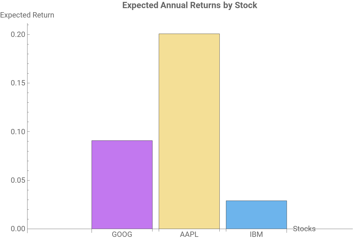
This function just substitutes the value of the “return” variable to work out the expected return.
In[]:=
expectedReturn=Exp[return*holdDays]-1
Out[]=
{{0.090908},{0.200842},{0.0289396}}
This produces a visual representation of the expected returns .
In[]:=
BarChart[Flatten[expectedReturn],ChartLabels->stockList,ChartStyle->"Pastel",BarOrigin->Bottom,ImageSize->Large,PlotLabel->Style["Expected Annual Returns by Stock",14,Bold],AxesLabel->{"Stocks","Expected Return"},LabelStyle->Directive[FontSize->12]]
Out[]=
3.3.2 Covariance
3.3.2 Covariance
The covariance matrix tells how 2 different stocks change together, therefore this helps us understand the risk & portfolio diversification between different stocks in the portfolio. This relationship analysis is fundamental to modern portfolio theory, as it allows investors to identify which assets move in harmony or opposition to each other, enabling the construction of diversified portfolios that can reduce overall risk while maintaining desired return levels through strategic asset allocation.
This Module function, defines all the values locally to the cell allowing the respective calculations to be done.
computeCovariance[stockSymbols_List,dates_List]:=Module[{holdDays,timeSeries,stockPrices,dailyDifferences,nObs,λ=0.94,weights,weightedMeanReturns,demeanedReturns,dailyDifferencesCovarianceEWMA,covariance},holdDays=252;timeSeries=FinancialData[#,dates]&/@stockSymbols;stockPrices=Table[Normal[QuantityMagnitude[timeSeries[[i]]]][[All,2]],{i,Length[timeSeries]}];dailyDifferences=Table[Differences[Log[stockPrices[[i]]]],{i,Length[stockPrices]}];nObs=Length[First[dailyDifferences]];weights= (1-λ)*λ ^Range[0,nObs-1];weights= weights / Total[weights];weightedMeanReturns=Dot[weights,Transpose[dailyDifferences]];demeanedReturns= Transpose[dailyDifferences]- Table[weightedMeanReturns,{nObs}];dailyDifferencesCovarianceEWMA = Dot[Transpose[demeanedReturns],(weights*demeanedReturns)];covariance= dailyDifferencesCovarianceEWMA*holdDays;covariance]
In[]:=
covarianceMatrix=computeCovariance[stockList,dates]
Out[]=
{{0.0954777,0.09214,0.0642504},{0.09214,0.143357,0.0768139},{0.0642504,0.0768139,0.11596}}
This function produces a visual representation for the covariance. The larger spheres show the stock with higher individual variance (more volatile), however, the smaller sphere should stocks with lower variance (more stable). Moreover the thicker lines show stronger correlation (positive or negative) on the other hand the thinner lines show weaker correlation. Claude was used to produce some of the code below.
In[]:=
covarianceMatrixForPlot=covarianceMatrix;{eigenVals,eigenVecs}=Eigensystem[N[covarianceMatrixForPlot]];
3D positions on a sphere instead of circle.
angles=N[Range[0,2Pi,2Pi/Length[stockList]]][[;;Length[stockList]]];radiusScale=3;positions3D=Table[radiusScale*{Cos[angles[[i]]],Sin[angles[[i]]],0.5*Sin[2*angles[[i]]]},{i,Length[stockList]}];
Colors based on diagonal variance.
colors=ColorData["Rainbow"]/@Rescale[Diagonal[covarianceMatrixForPlot],MinMax[Diagonal[covarianceMatrixForPlot]],{0,1}];
3D nodes with varying sizes based on variance.
3D edges with thickness variation.
3D Graphics with simple lighting
3.3.3 Maximum Allocation
3.3.3 Maximum Allocation
This takes the list of stocks requested by the user and returns a list of {1}s, to set the upper bound for the portfolio. This constraint mechanism is essential for practical portfolio management as it prevents over-concentration in any single asset, ensuring that the optimization algorithm maintains reasonable diversification limits and adheres to real-world investment guidelines that protect against excessive risk exposure to individual securities.
4. Equation Breakdown
4. Equation Breakdown
5. Plotting the Efficient Frontier Curve
5. Plotting the Efficient Frontier Curve
Here, I worked out all the key coordinates for the mean variance frontier plot. This visualization is critical for investors as it graphically represents the trade-off between risk and return across all possible portfolio combinations, allowing them to identify the optimal investment strategy that maximizes expected returns for a given level of risk tolerance or minimizes risk for a desired return target.
This calculates the investment weights as instructed by the minimum variance portfolio.
This calculates the investment weights as instructed by the naturally efficient portfolio .
This calculates the expected return of the minimum variance portfolio.
This calculates the expected return of the minimum variance portfolio using the dot product of portfolio weights and expected returns .
This calculates the expected return of the naturally efficient portfolio using the dot product of portfolio weights and expected returns .
This calculates the variance of the minimum variance portfolio using the quadratic form of portfolio weights and the covariance matrix .
This calculates the variance of the naturally efficient portfolio using the quadratic form of portfolio weights and the covariance matrix.
This calculates the covariance between the minimum variance portfolio and the naturally efficient portfolio using the cross
product of their respective weights and the covariance matrix.
product of their respective weights and the covariance matrix.
This is the visual representation of the mean frontier curve to visualize the different points & allowing users to understand different points of investment.
6. Additional Analyses of Different Portfolios
6. Additional Analyses of Different Portfolios
To try my tool out, I utilized top up voted/commented stock portfolio combinations on the reddit r/stocks. For that matter I created a function called meanVarianceFrontierAnalysis, which executes all the analytical steps outlined in the previous sections of the essay.
This function outputs the key parts of the code & visualizations for a user to quickly put there stocks in & get a output. This streamlined interface design prioritizes user experience by eliminating technical complexity and providing immediate, actionable insights, making sophisticated portfolio optimization accessible to investors regardless of their programming background while delivering professional-grade financial analysis in an intuitive format.
6.1 Portfolio 1
6.1 Portfolio 1
These are outputs from calling the meanVarianceFrontierAnalysis function over a list of stocks and dates to sample time series data.
The efficient frontier analysis reveals a significant deterioration in risk-adjusted returns between the two portfolio points. Point 1 (σ = 0.05, μ = 0.20) exhibits a Sharpe ratio of 4.00, while Point 2 (σ = 0.10, μ = 0.24) demonstrates a substantially inferior Sharpe ratio of 2.40, indicating markedly weaker risk-adjusted performance despite marginally higher absolute returns.The incremental risk-return ratio between these points is 0.80, suggesting that each additional unit of risk generates only 0.80 units of expected return, representing poor risk compensation. While Point 2 offers slightly higher absolute returns, the dramatic reduction in risk-adjusted performance makes Point 1 significantly more attractive from an efficiency standpoint. The investment decision strongly favors Point 1, as it provides exceptional risk-adjusted returns that are difficult to justify abandoning for the modest absolute return increase offered by Point 2. Point 1 represents superior compensation per unit of risk assumed, making it the clear optimal choice for rational investors seeking efficient portfolio construction.
Now, I will call my meanVarianceFrontierAnalysis tool to analyse portfolios over different choices of stocks and dates for which to retrieve time series data.
6.2 Portfolio 2
6.2 Portfolio 2
The efficient frontier analysis reveals a significant deterioration in risk-adjusted returns between the two portfolio points. Point 1 (σ = 0.15, μ = 0.18) exhibits a Sharpe ratio of 1.20, while Point 2 (σ = 0.25, μ = 0.38) demonstrates an inferior Sharpe ratio of 1.52, indicating improved risk-adjusted performance with higher absolute returns. The incremental risk-return ratio between these points is 2.00, suggesting that each additional unit of risk generates 2.00 units of expected return, representing favorable risk compensation. While Point 1 offers lower absolute returns, Point 2 provides both higher absolute returns and superior risk-adjusted performance, making it the more attractive choice from an efficiency standpoint. The investment decision favors Point 2, as it delivers better compensation per unit of risk assumed along with substantially higher expected returns. Point 2 represents superior risk-adjusted returns and absolute performance, making it the optimal choice for investors seeking efficient portfolio construction with enhanced return potential.
6.3 Portfolio 3
6.3 Portfolio 3
The efficient frontier analysis reveals a deterioration in risk-adjusted returns between the two portfolio points. Point 1 (σ = 0.05, μ = 0.10) exhibits a Sharpe ratio of 2.00, while Point 2 (σ = 0.15, μ = 0.20) demonstrates an inferior Sharpe ratio of 1.33, indicating weaker risk-adjusted performance despite higher absolute returns. The incremental risk-return ratio between these points is 1.00, it suggests that each additional unit of risk generates exactly 1.00 units of expected return. While Point 2 offers higher absolute returns, the reduced risk-adjusted performance makes Point 1 more attractive from an efficiency standpoint, though the investment decision ultimately depends on individual risk tolerance and return objectives. Both points present reasonable risk-return profiles on the efficient frontier, but Point 1 offers superior compensation per unit of risk assumed, making it the preferred choice for risk-conscious investors seeking optimal risk-adjusted returns.
6.4 Portfolio 4
6.4 Portfolio 4
The efficient frontier analysis reveals a deterioration in risk-adjusted returns between the two portfolio points. Point 1 (σ = 0.10, μ = 0.20) exhibits a Sharpe ratio of 2.00, while Point 2 (σ = 0.15, μ = 0.25) demonstrates an inferior Sharpe ratio of 1.67, indicating weaker risk-adjusted performance despite higher absolute returns. The incremental risk-return ratio between these points is 1.00, suggesting that each additional unit of risk generates exactly 1.00 units of expected return. While Point 2 offers higher absolute returns,the reduced risk-adjusted performance makes Point 1 more attractive from a efficiency standpoint, though the investment decision ultimately depends on individual risk tolerance and return objectives. Both points present reasonable risk-return profiles on the efficient frontier, but Point 1 offers superior compensation per unit of risk assumed.
7. Conclusions, Limitations & Future Work
7. Conclusions, Limitations & Future Work
In this project, stock portfolio optimization was analyzed through the lens of classical financial theory, specifically examining the mean-variance frontier framework and its underlying assumptions in order to find the optimal allocation of different assets in portfolio construction. This project involved critically evaluating the foundational principles of Modern Portfolio Theory, including the assumptions of rational investors, normal return distributions, and static correlation structures, while applying these models to equity-only allocations and eventually more complex multi-asset portfolios. Using classical financial theory frameworks, this project was able to demonstrate both the strengths and limitations of traditional theoretical approaches in practice, examining how established financial models perform in 2-D visualizations and 3-D classical financial theory models when confronted with real market data. Overall, this project aimed to bridge the gap between classical financial theory and practical portfolio management, investigating how traditional assumptions about market efficiency and investor behavior hold up against real-world market dynamics, and exploring the applicability of these theoretical frameworks to modern portfolio management strategies used in hedge funds as well as in retirement planning.
While this project did use mean-variance optimization to draw insights about the allocations of different assets in different market conditions, it also had a few notable limitations. These limitations include the lack of market fluctuation modeling in the optimization framework, particularly noticeable in the inability to capture dynamic market volatility and regime changes, the focus on static mean-variance analysis versus other types of optimization such as behavioral-driven models (more applicable to real investor psychology) and time-varying approaches (since most market conditions change over time). Another limitation is the restricted scope of the 3-D covariance model, which included a limited range of stocks rather than a comprehensive market representation, as well as the incomplete nature of the dataset used, which was not inclusive of all available securities in the market.
Further work should focus on addressing these limitations as well as expanding on the more basic approach used in this project. There is room for incorporating market fluctuation modeling techniques such as GARCH models or regime-switching frameworks to better capture market dynamics. Additionally, the project could expand to include a greater range of stocks in the 3-D covariance model, utilize more comprehensive datasets that encompass broader market coverage, and implement dynamic rebalancing strategies that account for changing market conditions, goals which were not possible in the time frame allotted for this project but which would have more real-world applications in portfolio management.
Acknowledgements
Acknowledgements
I want to thank to my mentor Carlos Angulo Zumaeta & the Directors of WSRP for there continuous support and guidance through my project . As well as Stephen Wolfram for helping me with the initial ideation & brainstorming process.
References
References
◼
Galichère, Arthur. EC333: Topics in Financial Economics–Theories and International Finance. University of Warwick, Department of Economics. Accessed 8th July 2025.
◼
Kumar, Manoj. Simple Returns vs. Log Returns: A Comprehensive Comparative Analysis for Financial Analysis, August 5th 2023.
◼
Lo, Andrew. Financial Theory 2 . Massachusetts Institute of Technology. MIT OpenCourseWare, https://ocw.mit.edu, August 2008.