Double Pareto lognormal distribution.
by R. H. Rimmer, 7 August 2024
by R. H. Rimmer, 7 August 2024
This is an old package written in 2011, which I decided to place in the public domain. At some point perhaps it will be added to Wolfram Language statistics functions. If you place the DPLN.m in the directory below, it should load properly.
In[]:=
FileNameJoin[$BaseDirectory,"Applications"]
Out[]=
C:\ProgramData\Wolfram\Applications
In[]:=
Needs["DPLN`"]
There are three distributions in the package there is a short name and a long name for each. The documentation is in the sections below.
In[]:=
Names["DPLN`*"]
Out[]=
{ALDistribution,AsymmetricLaplaceDistribution,DoubleParetoLogNormalDistribution,DPLNDistribution,NLDistribution,NormalLaplaceDistribution}
DoubleParetoLogNormalDistribution
DoubleParetoLogNormalDistribution
In[]:=
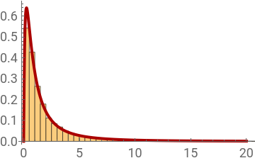
{a,b,d,c}={1.8,2,0,1};s=RandomVariate[DPLNDistribution[a,b,d,c],10000];h0=Histogram[s,Automatic,"PDF"];g1=Plot[PDF[DPLNDistribution[a,b,d,c],x],{x,0,20},PlotRangeAll,PlotStyle{Thick,Darker[Red]}];Show[h0,g1,PlotRange{{0,20},All}]
Out[]=
In[]:=
EstimatedDistribution[s,DPLNDistribution[α,β,μ,σ]]
Out[]=
DoubleParetoLogNormalDistribution[1.66951,1.94621,-0.0310658,0.964755]
In[]:=
FindDistributionParameters[s,DPLNDistribution[α,β,μ,σ]]
Out[]=
{α1.66951,β1.94621,μ-0.0310658,σ0.964755}
NormalLaplaceDistribution
NormalLaplaceDistribution
In[]:=
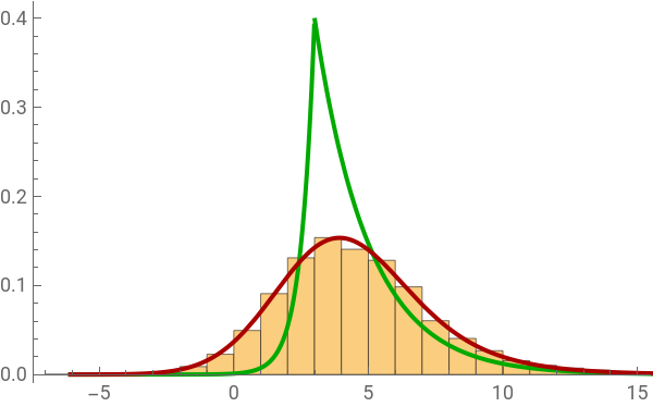
{a,b,d,c}={0.5,2,3,2};s=RandomVariate[NormalLaplaceDistribution[a,b,d,c],10000];h0=Histogram[s,Automatic,"PDF"];g0=Plot[PDF[AsymmetricLaplaceDistribution[a,b],x-d],{x,Min[s],Max[s]},PlotRangeAll,PlotStyle{Thick,Darker[Green]}];g1=Plot[PDF[NLDistribution[a,b,d,c],x],{x,Min[s],Max[s]},PlotRangeAll,PlotStyle{Thick,Darker[Red]}];Show[h0,g0,g1]
Out[]=
In[]:=
EstimatedDistribution[s,NLDistribution[α,β,μ,σ]]
Out[]=
NormalLaplaceDistribution[0.466054,1.36828,3.13383,1.84036]
In[]:=
FindDistributionParameters[s,NLDistribution[α,β,μ,σ]]
Out[]=
{α0.466054,β1.36828,μ3.13383,σ1.84036}
In[]:=
Mean[s]Mean[NLDistribution[0.5,2,3,2]]Mean[NLDistribution[α,β,μ,σ]]
Out[]=
4.54863
Out[]=
4.5
Out[]=
1
α
1
β
In[]:=
StandardDeviation[s]StandardDeviation[NLDistribution[0.5,2,3,2]]StandardDeviation[NLDistribution[α,β,μ,σ]]
Out[]=
2.91817
Out[]=
2.87228
Out[]=
1
2
α
1
2
β
2
σ
AsymmetricLaplaceDistribution
AsymmetricLaplaceDistribution
In[]:=
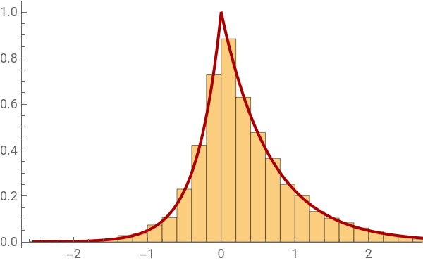
s=RandomVariate[AsymmetricLaplaceDistribution[1.5,3],10000];h0=Histogram[s,30,"PDF"];g0=Plot[PDF[AsymmetricLaplaceDistribution[1.5,3],x],{x,Min[s],Max[s]},PlotRangeAll,PlotStyle{Thick,Darker[Red]}];Show[h0,g0]
Out[]=
In[]:=
Mean[s]Mean[AsymmetricLaplaceDistribution[1.5,3]]Mean[AsymmetricLaplaceDistribution[α,β]]
Out[]=
0.330392
Out[]=
0.333333
Out[]=
-α+β
αβ
There is an abbreviation to save typing.
In[]:=
StandardDeviation[s]StandardDeviation[ALDistribution[1.5,3]]StandardDeviation[ALDistribution[α,β]]
Out[]=
0.743048
Out[]=
0.745356
Out[]=
1
2
α
1
2
β
In[]:=
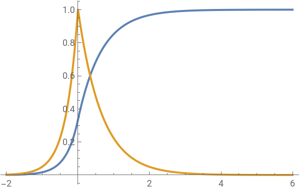
ed=EstimatedDistribution[s,ALDistribution[α,β]]Plot[{CDF[ed,x],PDF[ed,x]},{x,-2,6},PlotRangeAll]
Out[]=
AsymmetricLaplaceDistribution[1.5061,2.99784]
Out[]=
William Reed developed these distributions there are papers available at his web site: http://www.math.uvic.ca/faculty/reed/