Recovering Antoine Equation Parameters for Benzene via Particle Swarm Optimization
Housam Binous
Recovering Antoine Equation Parameters for Benzene via Particle Swarm Optimization
Housam Binous
Housam Binous
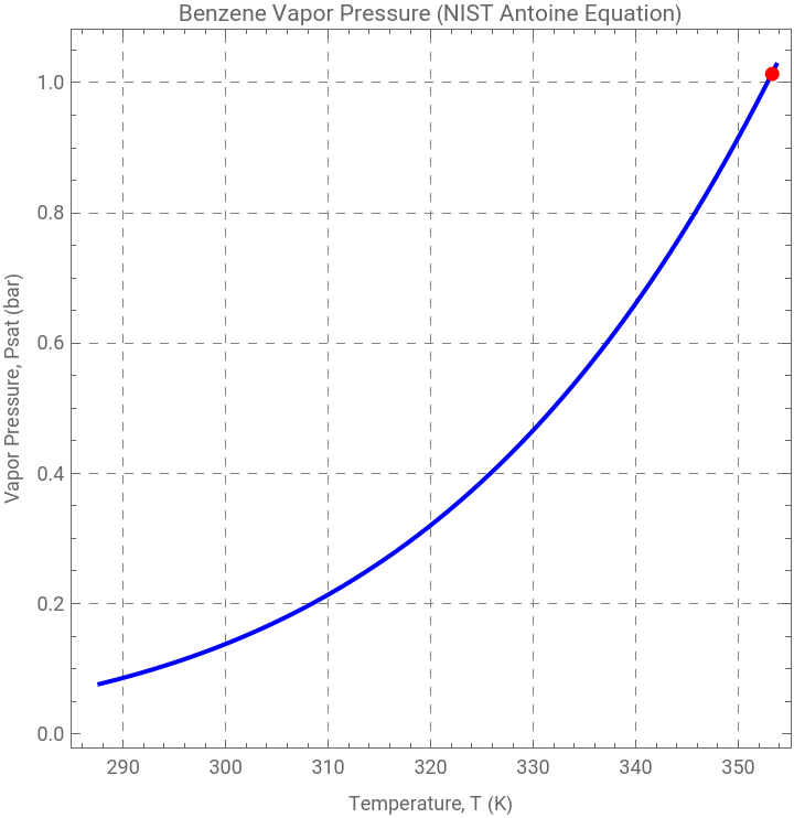
This Mathematica notebook applies particle swarm optimization to recover the Antoine equation constants for benzene from synthetic “experimental” data, rather than simply plugging in literature values. The first section regenerates the reference vapor pressure table using the known NIST coefficients (A = 4.01814, B = 1203.835, C = −53.226, valid from 287.70 K to 354.07 K), computes Psat at each temperature, and plots the resulting curve. This table — stored in t1 — is then treated as the “experimental” dataset that the PSO algorithm will later try to fit, with the normal boiling point (353.3 K, 1.01325 bar) marked on the plot as a check.
The core of the notebook defines a Fitness[{A_, B_, C_}] function that measures how well a candidate set of Antoine parameters reproduces the experimental log-pressure values: it computes the sum of squared errors between log10 of the model prediction and log10 of the tabulated data across every temperature point in t1. The psoOptimize function is the swarm-based optimizer — particles representing candidate (A, B, C) triples are initialized randomly within bounds (FitnessLB = -200, FitnessUB = 1500), then iteratively updated using inertia (w = 0.72984), cognitive (c1 = 1.42), and social (c2 = 1.42) terms pulling each particle toward its own best-found position and the swarm’s global best. Because the search space here is genuinely 3-dimensional (one dimension per Antoine constant) and the bounds are wide, the swarm size and iteration count were both increased (150 particles, up to 2000 iterations) to ensure convergence to a precise minimum.
The results validate the approach well: after 2000 iterations the loss collapses from roughly 3×10⁻⁴ down to about 1.18×10⁻⁷, and the PSO-recovered parameters — A ≈ 4.0093, B ≈ 1199.14, C ≈ −53.74 — closely match the literature values (4.01814, 1203.835, −53.226) used to generate the synthetic data in the first place. This is a nice closed-loop demonstration: it confirms that PSO can successfully solve a nonlinear least-squares curve-fitting problem (recovering Antoine constants) purely through swarm-based search, without gradients or an analytical solution, and the close agreement between recovered and “true” constants serves as a built-in correctness check on both the optimizer and the fitness function.
In[]:=
(*NISTAntoineEquationforBenzene*)(*log10(P)=A-(B/(T+C)),Pinbar,TinK*)(*Source:Williamham,Taylor,etal.,1945(NISTWebBook)*)(*Validrange:287.70Kto354.07K*)Aant=4.01814;Bant=1203.835;Cant=-53.226;PsatBenzene[Tk_]:=10^(Aant-Bant/(Tk+Cant));(*GenerateTvsPsatdatatable*)TKmin=287.70;TKmax=354.07;t1=Table[{Tk,PsatBenzene[Tk]},{Tk,TKmin,TKmax,1}];(*Displayasaformattedtablecalled*)TableForm[t1,TableHeadings->{None,{"T (K)","Psat (bar)"}}]
Out[]//TableForm=
T (K) | Psat (bar) |
287.7 | 0.0765501 |
288.7 | 0.0804914 |
289.7 | 0.0845997 |
290.7 | 0.0888804 |
291.7 | 0.0933391 |
292.7 | 0.0979813 |
293.7 | 0.102813 |
294.7 | 0.10784 |
295.7 | 0.113068 |
296.7 | 0.118503 |
297.7 | 0.124153 |
298.7 | 0.130022 |
299.7 | 0.136117 |
300.7 | 0.142446 |
301.7 | 0.149014 |
302.7 | 0.155829 |
303.7 | 0.162897 |
304.7 | 0.170226 |
305.7 | 0.177822 |
306.7 | 0.185694 |
307.7 | 0.193848 |
308.7 | 0.202291 |
309.7 | 0.211033 |
310.7 | 0.22008 |
311.7 | 0.22944 |
312.7 | 0.239122 |
313.7 | 0.249133 |
314.7 | 0.259482 |
315.7 | 0.270177 |
316.7 | 0.281226 |
317.7 | 0.292639 |
318.7 | 0.304423 |
319.7 | 0.316588 |
320.7 | 0.329143 |
321.7 | 0.342097 |
322.7 | 0.355458 |
323.7 | 0.369237 |
324.7 | 0.383443 |
325.7 | 0.398085 |
326.7 | 0.413172 |
327.7 | 0.428715 |
328.7 | 0.444724 |
329.7 | 0.461208 |
330.7 | 0.478178 |
331.7 | 0.495643 |
332.7 | 0.513615 |
333.7 | 0.532102 |
334.7 | 0.551117 |
335.7 | 0.57067 |
336.7 | 0.590771 |
337.7 | 0.611431 |
338.7 | 0.632661 |
339.7 | 0.654472 |
340.7 | 0.676876 |
341.7 | 0.699883 |
342.7 | 0.723505 |
343.7 | 0.747754 |
344.7 | 0.77264 |
345.7 | 0.798176 |
346.7 | 0.824374 |
347.7 | 0.851244 |
348.7 | 0.8788 |
349.7 | 0.907052 |
350.7 | 0.936014 |
351.7 | 0.965696 |
352.7 | 0.996113 |
353.7 | 1.02728 |
In[]:=
(*PlotPsatvsT*)plt1=ListPlot[t1,Joined->True,PlotStyle->{Blue,Thick},Frame->True,FrameLabel->{"Temperature, T (K)","Vapor Pressure, Psat (bar)"},PlotLabel->"Benzene Vapor Pressure (NIST Antoine Equation)",GridLines->Automatic,GridLinesStyle->Directive[Gray,Dashed],AspectRatio->1];(*Normalboilingpointisidentifiedbythereddotforreference:T=353.3K,P=1.01325bar*)plt2=Show[plt1,Graphics[{Red,PointSize[0.02],Point[{353.3,1.01325}]}],Epilog->{Text["NBP: 353.3 K, 1 atm",{353.3,1.01325},{-1.2,-1}]}]
Out[]=
In[]:=
SwarmDim=3;(*3Dproblem*)(*upperandlowerboundsfothesearchdomain*)FitnessLB=-200;FitnessUB=1500;c1=1.42;c2=1.42;w=0.72984;(*psoparameters*)T=Table[i,{i,TKmin,TKmax,1}];(*t1willconstitute/mimicourexperimentalpoints*)Fitness[{A_,B_,C_}]:=Sum[((A-B/(T[[i]]+C))-Log[10,t1[[i]][[2]]])^2,{i,1,Length@T}];
In[]:=
(*PSOOptimizer*)psoOptimize[lossFunc_,dim_,lb_,ub_,nParticles_:150,nIter_:1000,w_:0.72984,c1_:2,c2_:2]:=Module[{particles,velocities,pbest,pbestScore,gbest,gbestScore,convergence={},r1,r2,score,gbestIdx},(*Initializeparticlesuniformlywithin[lb,ub]ineachdimension*)particles=RandomReal[{lb,ub},{nParticles,dim}];velocities=ConstantArray[0.,{nParticles,dim}];pbest=particles;pbestScore=Table[lossFunc[particles[[i]]],{i,nParticles}];gbestIdx=First@Ordering[pbestScore,1];gbestScore=pbestScore[[gbestIdx]];gbest=pbest[[gbestIdx]];Do[Do[r1=RandomReal[1,dim];r2=RandomReal[1,dim];velocities[[i]]=w*velocities[[i]]+c1*r1*(pbest[[i]]-particles[[i]])+c2*r2*(gbest-particles[[i]]);particles[[i]]+=velocities[[i]];(*keepparticleswithinbounds*)particles[[i]]=Clip[particles[[i]],{lb,ub}];score=lossFunc[particles[[i]]];If[score<pbestScore[[i]],pbest[[i]]=particles[[i]];pbestScore[[i]]=score;];,{i,nParticles}];gbestIdx=First@Ordering[pbestScore,1];gbestScore=pbestScore[[gbestIdx]];gbest=pbest[[gbestIdx]];AppendTo[convergence,gbestScore];If[Mod[t,50]==0,Print["PSO Iter ",t," Loss = ",gbestScore]];,{t,nIter}];{gbest,gbestScore,convergence}];(*RunPSO*){bestPos,bestScore,convergence}=psoOptimize[Fitness,SwarmDim,FitnessLB,FitnessUB,500,2000,w,c1,c2];Print["Best position: ",bestPos];Print["Best fitness: ",bestScore];