This is the first part of post series that serve as a concise guide to harnessing the possibilities of the Wolfram plugin for mathematics, physics and Wolfram Language coding, with a special focus on effective problem-solving prompting techniques, exemplified with 100+ plugin-using ChatGPT chat sessions.
Check out other parts of this guide here:
Guide 1: https://community.wolfram.com/groups/-/m/t/3070428
Guide 2: https://community.wolfram.com/groups/-/m/t/3075538
Guide 3: https://community.wolfram.com/groups/-/m/t/3077476
Guide 4: https://community.wolfram.com/groups/-/m/t/3077667
Guide 1: https://community.wolfram.com/groups/-/m/t/3070428
Guide 2: https://community.wolfram.com/groups/-/m/t/3075538
Guide 3: https://community.wolfram.com/groups/-/m/t/3077476
Guide 4: https://community.wolfram.com/groups/-/m/t/3077667
Contents
Contents
Plugin Usage Examples Writing Wolfram Language Code Making Datasets Writing Wolfram Language Code Using ChatGPT’s Background Knowledge Predicting Wolfram Language Code Results Not Perfect Code, but Still Quite Useful Guiding ChatGPT through a Computation (Is This the Future?) Changing/Improving/Commenting /Explaining Wolfram Language Code Just Having Some Fun Trust, But Verify Missing Intuition Reproducibility Plain FailuresThe Next Step: Programmatic LLM Uses Motivation Two ExamplesSummary Prompts Wolfram Plugin LLMSynthesize
Cell coloring conventions
Cell coloring conventions
Plugin Usage Examples
Plugin Usage Examples
Writing Wolfram Language Code
Writing Wolfram Language Code
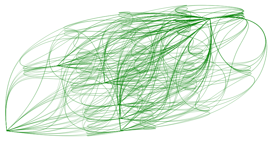
Partial sum curves
Partial sum curves
User prompt:
Take six random numbers from the unit circle. Form all possible permutations of these lists.
For each list form the partial sums and represent each sequence of partial sums as a B-spline curve.
Show all these curves together as thin, slightly transparent dark green curves.
Explain the steps to code this up and show the final code.
Take six random numbers from the unit circle. Form all possible permutations of these lists.
For each list form the partial sums and represent each sequence of partial sums as a B-spline curve.
Show all these curves together as thin, slightly transparent dark green curves.
Explain the steps to code this up and show the final code.

In[]:=
(*Step1:Generate6randompointsontheunitcircle*)randomPointsOnUnitCircle[n_]:=Table[{Cos[#],Sin[#]}&@RandomReal[{0,2*Pi}],{n}];(*Step2:Generateallpermutations*)allPermutations[points_]:=Permutations[points];(*Step3:Computepartialsums*)partialSums[points_]:=Accumulate[points];(*Step4&5:GenerateB-splinecurvesandvisualize*)visualizeBSplineCurves[pointsList_]:=Graphics[{{Thin,Darker[Green,0.5],Opacity[0.5],BSplineCurve[partialSums[#]]}&/@pointsList},Axes->False];(*Mainfunctiontocombineallsteps*)generateAndVisualizeBSplines[n_]:=Module[{points,perms},points=randomPointsOnUnitCircle[n];perms=allPermutations[points];visualizeBSplineCurves[perms]];(*Callthemainfunction*)generateAndVisualizeBSplines[6]
Out[]=
Clock face
Clock face
User prompt:
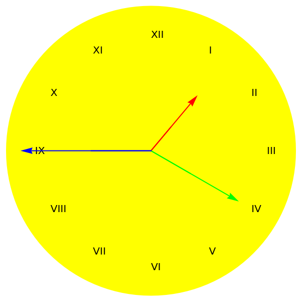
Please write me code that plots an elegant clock. I want a hour, minute, second hand and Roman numerals for the hours.
Each hand (with an arrow please) in a different color, yellow face of the clock. Let the hour, minute, second be the arguments of the function.
Please test that the hands point in the correct direction.
Please write me code that plots an elegant clock. I want a hour, minute, second hand and Roman numerals for the hours.
Each hand (with an arrow please) in a different color, yellow face of the clock. Let the hour, minute, second be the arguments of the function.
Please test that the hands point in the correct direction.
clockPlot[hour_,minute_,second_]:=Module[{hourHand,minuteHand,secondHand,numerals,numeralPositions,numeralLabels,clockFace},(*Definethehandsoftheclock*)hourHand=Line[{{0,0},0.5{Cos[Pi/2-2Pi(hour+minute/60)/12],Sin[Pi/2-2Pi(hour+minute/60)/12]}}];minuteHand=Line[{{0,0},0.7{Cos[Pi/2-2Piminute/60],Sin[Pi/2-2Piminute/60]}}];secondHand=Line[{{0,0},0.9{Cos[Pi/2-2Pisecond/60],Sin[Pi/2-2Pisecond/60]}}];(*DefinetheRomannumerals*)numerals={"XII","I","II","III","IV","V","VI","VII","VIII","IX","X","XI"};numeralPositions=Table[0.8{Cos[Pi/2-2Pii/12],Sin[Pi/2-2Pii/12]},{i,0,11}];numeralLabels=Table[Text[numerals[[i+1]],numeralPositions[[i+1]],{-1,0}],{i,0,11}];(*Definetheclockface*)clockFace=Disk[{0,0},1];(*Plottheclock*)Graphics[{Yellow,clockFace,Black,numeralLabels,Red,Arrow[hourHand],Green,Arrow[minuteHand],Blue,Arrow[secondHand]},ImageSize->300]];
(*Testthefunctionwithaspecifictime:3:15:45*)clockPlot[1,20,45]
Out[]=
Berggren Pythagorean triples
Berggren Pythagorean triples
Linear regression with uncertainties
Linear regression with uncertainties
Continued fraction of Champernowne primes
Continued fraction of Champernowne primes
Random walk on a sphere
Random walk on a sphere
User prompt:
My end goal is a fancy 3D graphics.
The first step would be to model a random walk on a sphere.
At each step go a fixed constant distance in a randomly selected direction.
Write a program that does n steps. Explain how it works.
Show the code.
Don’t run anything.
Now comes step two:
Make a 200 step random walk of step length 0.2.
Then make lets make the magnitude (radius) of the n-th point of the resulting list be n*0.2.
Finally make a 3D graphics of a orange tube through all points.
Just show the code again.
No need to run it.
My end goal is a fancy 3D graphics.
The first step would be to model a random walk on a sphere.
At each step go a fixed constant distance in a randomly selected direction.
Write a program that does n steps. Explain how it works.
Show the code.
Don’t run anything.
Now comes step two:
Make a 200 step random walk of step length 0.2.
Then make lets make the magnitude (radius) of the n-th point of the resulting list be n*0.2.
Finally make a 3D graphics of a orange tube through all points.
Just show the code again.
No need to run it.
User prompt:
In the following every time I input a task, I want you
1)) develop and display well-documented Wolfram Language code that solves the problem
and display it in a terminal-like way with proper line length
2) evaluate the code on the Wolfram Language API (remember the formatting rules for this API)
3) display the result returned from the Wolfram Language API
Consider this map m(alpha) from Z2 to Z2: {m,n}->{floor(alpha m)-n,m};
Implement a function that given given alpha and an initial {n,m} find a complete cycle, meaning all values {m’,n’} that arise from the application of the map until the values {m,n} are reached again.
Test the function an alpha=2/5, {m_start,n_start}={1,3}
In the following every time I input a task, I want you
1)) develop and display well-documented Wolfram Language code that solves the problem
and display it in a terminal-like way with proper line length
2) evaluate the code on the Wolfram Language API (remember the formatting rules for this API)
3) display the result returned from the Wolfram Language API
Consider this map m(alpha) from Z2 to Z2: {m,n}->{floor(alpha m)-n,m};
Implement a function that given given alpha and an initial {n,m} find a complete cycle, meaning all values {m’,n’} that arise from the application of the map until the values {m,n} are reached again.
Test the function an alpha=2/5, {m_start,n_start}={1,3}
Random disk collection eigenfunctions
Random disk collection eigenfunctions
User prompt:
Take 60 random unit disks with centers randomly distributes between -4 and 4 in x and y direction. Form the region union of these disks.
Then, write well-documented Wolfram Language code to
1) numerically compute the 20th eigenfunction of the negative Laplace operator (in 2D) on this region union. Assume Dirichlet boundary conditions on all boundaries.
2) make a high-res 3D plot of this eigenfunction with mesh lines according to the function values.
3) make a high-res contour plot of this eigenfunction with values <=0 in blue and values > 0 in red.
Take 60 random unit disks with centers randomly distributes between -4 and 4 in x and y direction. Form the region union of these disks.
Then, write well-documented Wolfram Language code to
1) numerically compute the 20th eigenfunction of the negative Laplace operator (in 2D) on this region union. Assume Dirichlet boundary conditions on all boundaries.
2) make a high-res 3D plot of this eigenfunction with mesh lines according to the function values.
3) make a high-res contour plot of this eigenfunction with values <=0 in blue and values > 0 in red.
Gauss–Lucas theorem visualization
Gauss–Lucas theorem visualization
User prompt:
I was thinking on a visualization of the Gauss-Lucas theorem:
Start with a degree 40 polynomial with each coefficient a random complex number from the unit disk.
Then for the n-time differentiated polynomial get its roots. Then show the roots as points and the outer boundary of the convex hull (not the interior) of the roots (use RegionBoundary[ConvexHullMesh[...]] for this step).
Show these points and the outer boundary of the convex hull for n=0, 1, 2, 3, ..., 20.
Show them all together in one plot.
Explain the way to get the convex hull and show the final Wolfram Language code.
Please write the code in a modular manner and and test each of the functions before implementing the next one.
In the beginning let’s make a plan of the functions to be implemented, their arguments and the structure/type of their outputs. Differentiate between the roots as complex numbers and roots as pairs of {realPart, imaginaryPart}].
Make sure to always include all code in every API call.
I was thinking on a visualization of the Gauss-Lucas theorem:
Start with a degree 40 polynomial with each coefficient a random complex number from the unit disk.
Then for the n-time differentiated polynomial get its roots. Then show the roots as points and the outer boundary of the convex hull (not the interior) of the roots (use RegionBoundary[ConvexHullMesh[...]] for this step).
Show these points and the outer boundary of the convex hull for n=0, 1, 2, 3, ..., 20.
Show them all together in one plot.
Explain the way to get the convex hull and show the final Wolfram Language code.
Please write the code in a modular manner and and test each of the functions before implementing the next one.
In the beginning let’s make a plan of the functions to be implemented, their arguments and the structure/type of their outputs. Differentiate between the roots as complex numbers and roots as pairs of {realPart, imaginaryPart}].
Make sure to always include all code in every API call.
User prompt:
Can you make me a picture of a few sheets of the Riemann surface w(z) if w(z) is implicitly defined through
z = 2w - exp(w) + 1. Say Re(w) over the complex z-plane and Im(w) over the complex z-plane.
Don’t solve for w, this will be too complicated.
Can you think on a ‘clever’ way?
Hint: think backwards and use ParametricPlot3D
Can you make me a picture of a few sheets of the Riemann surface w(z) if w(z) is implicitly defined through
z = 2w - exp(w) + 1. Say Re(w) over the complex z-plane and Im(w) over the complex z-plane.
Don’t solve for w, this will be too complicated.
Can you think on a ‘clever’ way?
Hint: think backwards and use ParametricPlot3D
Writing Wolfram Language Code Using ChatGPT’s Background Knowledge
Writing Wolfram Language Code Using ChatGPT’s Background Knowledge
Relativistic velocity addition
Relativistic velocity addition
User prompt:
Implement a Wolfram Language function that implements the relativistic velocity addition law.
Show the implementation.
The function should take two 3D velocity vectors and return the resulting combined velocity vector.
Do not assume the two velocities point in the same direction, meaning take the Thomas-Wigner rotation into account.
Explicitly check (using the implemented formula on the API!!) that in the case of parallel velocities one recovers the classic (v_1x+v_2x)/(1+v_1x v2x_/c^2) for v_1= {0.3 c, 0,0} and v_2= {0.6 c, 0,0}.
Check that the implemented formula is symmetric in v1 and v2. Explain how to check the symmetry for generic v_1={v_1x, v_1y, v_1z}, v_2={v_2x, v_2y, v_2z}.
IMPORTANT: Explicitly show the code you use for the checks before running the checks!
Please also include a Wikipedia reference (with link) for the formula that you will use.
Do not cheat and implement the parallel situation as a special case of the formula.
Before starting recall for yourself the various forms of this addition law and select the most concise one.
Implement a Wolfram Language function that implements the relativistic velocity addition law.
Show the implementation.
The function should take two 3D velocity vectors and return the resulting combined velocity vector.
Do not assume the two velocities point in the same direction, meaning take the Thomas-Wigner rotation into account.
Explicitly check (using the implemented formula on the API!!) that in the case of parallel velocities one recovers the classic (v_1x+v_2x)/(1+v_1x v2x_/c^2) for v_1= {0.3 c, 0,0} and v_2= {0.6 c, 0,0}.
Check that the implemented formula is symmetric in v1 and v2. Explain how to check the symmetry for generic v_1={v_1x, v_1y, v_1z}, v_2={v_2x, v_2y, v_2z}.
IMPORTANT: Explicitly show the code you use for the checks before running the checks!
Please also include a Wikipedia reference (with link) for the formula that you will use.
Do not cheat and implement the parallel situation as a special case of the formula.
Before starting recall for yourself the various forms of this addition law and select the most concise one.
Quantum carpet
Quantum carpet
User prompt:
Could you provide me some code that makes a density plot of a so-called ‘quantum carpet’.
Let’s start with recalling what a ‘quantum carpet’ is and explicitly point out what makes it different from a simple
smooth time-evolution of a finite superposition of eigenfunctions.
I was thinking we would use the example of a finite square well in [0, pi] with initial conditions
psi(t=0) = 1/sqrt(pi).
Please develop the code step-by-step.
Explain each step and show me code for it.
As the final plot might be quite time-consuming, just provide me the code for the final plot.
Could you provide me some code that makes a density plot of a so-called ‘quantum carpet’.
Let’s start with recalling what a ‘quantum carpet’ is and explicitly point out what makes it different from a simple
smooth time-evolution of a finite superposition of eigenfunctions.
I was thinking we would use the example of a finite square well in [0, pi] with initial conditions
psi(t=0) = 1/sqrt(pi).
Please develop the code step-by-step.
Explain each step and show me code for it.
As the final plot might be quite time-consuming, just provide me the code for the final plot.
Predicting Wolfram Language Code Results
Predicting Wolfram Language Code Results
B-spline surface
B-spline surface
User prompt:
Explain what this code does:
With[{M = 100}, Graphics3D[{Purple, BSplineSurface[
Table[#[[Last[FindShortestTour[#]]]] &[RandomPoint[Ball[], M]], 3]]}]]
Explain what this code does:
With[{M = 100}, Graphics3D[{Purple, BSplineSurface[
Table[#[[Last[FindShortestTour[#]]]] &[RandomPoint[Ball[], M]], 3]]}]]
Summary
M random points are generated within a unit ball.
These points are reordered to form a path with the shortest possible total distance.
This process is repeated 3 times (due to Table[..., 3]), generating 3 lists of ordered points.
A B-spline surface is created using these 3 lists of points as control points.
The B-spline surface is rendered in a 3D graphic with a purple color.
The resulting graphic will show a smooth, purple B-spline surface that passes near the random points generated within the unit ball.
M random points are generated within a unit ball.
These points are reordered to form a path with the shortest possible total distance.
This process is repeated 3 times (due to Table[..., 3]), generating 3 lists of ordered points.
A B-spline surface is created using these 3 lists of points as control points.
The B-spline surface is rendered in a 3D graphic with a purple color.
The resulting graphic will show a smooth, purple B-spline surface that passes near the random points generated within the unit ball.
Logistic map
Logistic map
User prompt:
Please explain the following code.
Not just the at the function-by-function level, but also conceptually what this code tries to visualize and why this is interesting to visualize in the first place.
Before answering, think about the type of equations that the solves and how many solutions there are.
n = 6;
ode = D[iteratedLogisticMap[n, r][x[r]], r] // Simplify;
roots = SolveValues[ iteratedLogisticMap[n, Pi][x] == 0, x, Complexes];
Monitor[nds = Flatten[Table[x /. NDSolve[{ode == 0, x[Pi] == roots[[jk]]}, x, {r, 0, 8},
MaxSteps -> 1000], {jk, Length[roots]}]] // Quiet;,
Row[{“solving ODE #”, jk, “ from “, Length[roots]}]]
Show[{ParametricPlot3D[{Re[#[r]], Im[#[r]],
r}, {r, #[[1, 1, 1]], #[[1, 1, 2]]}, PlotStyle -> Thickness[0.002]] & /@ nds,
Graphics3D[{Opacity[0.3], Yellow,
Polygon[{{-2, -2, 4}, {2, -2, 4}, {2, 2, 4}, {-2, 2, 4}}]}]},
PlotRange -> {{-2, 2}, {-2, 2}, {0, 8}}, BoxRatios -> {1, 1, 0.6}]
Please explain the following code.
Not just the at the function-by-function level, but also conceptually what this code tries to visualize and why this is interesting to visualize in the first place.
Before answering, think about the type of equations that the solves and how many solutions there are.
n = 6;
ode = D[iteratedLogisticMap[n, r][x[r]], r] // Simplify;
roots = SolveValues[ iteratedLogisticMap[n, Pi][x] == 0, x, Complexes];
Monitor[nds = Flatten[Table[x /. NDSolve[{ode == 0, x[Pi] == roots[[jk]]}, x, {r, 0, 8},
MaxSteps -> 1000], {jk, Length[roots]}]] // Quiet;,
Row[{“solving ODE #”, jk, “ from “, Length[roots]}]]
Show[{ParametricPlot3D[{Re[#[r]], Im[#[r]],
r}, {r, #[[1, 1, 1]], #[[1, 1, 2]]}, PlotStyle -> Thickness[0.002]] & /@ nds,
Graphics3D[{Opacity[0.3], Yellow,
Polygon[{{-2, -2, 4}, {2, -2, 4}, {2, 2, 4}, {-2, 2, 4}}]}]},
PlotRange -> {{-2, 2}, {-2, 2}, {0, 8}}, BoxRatios -> {1, 1, 0.6}]
Summary
M random points are generated within a unit ball.
These points are reordered to form a path with the shortest possible total distance.
This process is repeated 3 times (due to Table[..., 3]), generating 3 lists of ordered points.
A B-spline surface is created using these 3 lists of points as control points.
The B-spline surface is rendered in a 3D graphic with a purple color.
The resulting graphic will show a smooth, purple B-spline surface that passes near the random points generated within the unit ball.
M random points are generated within a unit ball.
These points are reordered to form a path with the shortest possible total distance.
This process is repeated 3 times (due to Table[..., 3]), generating 3 lists of ordered points.
A B-spline surface is created using these 3 lists of points as control points.
The B-spline surface is rendered in a 3D graphic with a purple color.
The resulting graphic will show a smooth, purple B-spline surface that passes near the random points generated within the unit ball.
Periodic interlocking tiling
Periodic interlocking tiling
User prompt:
Here is some Wolfram Language coder that makes some pretty pattern.
First explain function by function what happens.
Then describe ‘philosophically’ what this code does and what are the special features of the resulting graphics.
curveCount = 6;
curvePointCount = 6;
squares = 3;
curvePoints = Table[With[{mp = RandomReal[ {0, 1}, 2]}, (mp + #) & /@ (RandomReal[{-1, 1},
{curvePointCount, 2}]/3)],
curveCount];
translatedCurves = Flatten[Flatten[Table[If[i == j == 0, Nothing, (# + {i, j}) & /@ #], {i, -1, 1}, {j, -1, 1}], 1] & /@ curvePoints, 1];
curveAnnotatedCurvePoints = Flatten[Table[
Table[bf = BSplineFunction[({i, j} + #) & /@ curvePoints[[k]], SplineDegree -> 4];
Table[bf[t] -> k, {t, 0, 1, 1/1200}], {i, -1, 1}, {j, -1, 1}],
{k, curveCount}]];
nf = Nearest[curveAnnotatedCurvePoints];
nearestToCurvek[{x_Real, y_Real}, k_] := nf[{x, y}] == {k}
regionCurvePairList = Table[
With[{col = RandomColor[]},
{RegionPlot[nearestToCurvek[{x, y}, k], {x, 0, 1}, {y, 0, 1},
PlotPoints -> 60, BoundaryStyle -> None, PlotStyle -> Lighter[col]],
Graphics[{col, Thick, BSplineCurve[curvePoints[[k]]]}]}], {k, curveCount}];
Graphics[{
Table[GeometricTransformation[regionCurvePairList[[k, 1, 1]],
TranslationTransform[{i, j}]], {k, curveCount}, {i, 0, squares}, {j, 0, squares}],
Table[GeometricTransformation[regionCurvePairList[[k, 2, 1]],
TranslationTransform[{i, j}]], {k, curveCount}, {i, 0, squares}, {j, 0, squares}]},
PlotRange -> {{0, squares}, {0, squares}}, PlotRangeClipping -> True]
Here is some Wolfram Language coder that makes some pretty pattern.
First explain function by function what happens.
Then describe ‘philosophically’ what this code does and what are the special features of the resulting graphics.
curveCount = 6;
curvePointCount = 6;
squares = 3;
curvePoints = Table[With[{mp = RandomReal[ {0, 1}, 2]}, (mp + #) & /@ (RandomReal[{-1, 1},
{curvePointCount, 2}]/3)],
curveCount];
translatedCurves = Flatten[Flatten[Table[If[i == j == 0, Nothing, (# + {i, j}) & /@ #], {i, -1, 1}, {j, -1, 1}], 1] & /@ curvePoints, 1];
curveAnnotatedCurvePoints = Flatten[Table[
Table[bf = BSplineFunction[({i, j} + #) & /@ curvePoints[[k]], SplineDegree -> 4];
Table[bf[t] -> k, {t, 0, 1, 1/1200}], {i, -1, 1}, {j, -1, 1}],
{k, curveCount}]];
nf = Nearest[curveAnnotatedCurvePoints];
nearestToCurvek[{x_Real, y_Real}, k_] := nf[{x, y}] == {k}
regionCurvePairList = Table[
With[{col = RandomColor[]},
{RegionPlot[nearestToCurvek[{x, y}, k], {x, 0, 1}, {y, 0, 1},
PlotPoints -> 60, BoundaryStyle -> None, PlotStyle -> Lighter[col]],
Graphics[{col, Thick, BSplineCurve[curvePoints[[k]]]}]}], {k, curveCount}];
Graphics[{
Table[GeometricTransformation[regionCurvePairList[[k, 1, 1]],
TranslationTransform[{i, j}]], {k, curveCount}, {i, 0, squares}, {j, 0, squares}],
Table[GeometricTransformation[regionCurvePairList[[k, 2, 1]],
TranslationTransform[{i, j}]], {k, curveCount}, {i, 0, squares}, {j, 0, squares}]},
PlotRange -> {{0, squares}, {0, squares}}, PlotRangeClipping -> True]
Philosophical Description:
The code artistically combines randomness with structure. It generates random B-spline curves and then creates Voronoi-like regions where each region corresponds to points nearest to a particular curve. The curves and their regions are then replicated across a grid, creating a repeating pattern with slight variations due to the randomness of the curves. The result is a mosaic of intertwined curves and regions, each with its unique color, producing a visually appealing and intricate pattern. The use of B-splines ensures smooth curves, and the translation across the grid provides a sense of order amidst the randomness. The graphics produced by this code exemplify the harmony between chaos and order, randomness and structure.
The code artistically combines randomness with structure. It generates random B-spline curves and then creates Voronoi-like regions where each region corresponds to points nearest to a particular curve. The curves and their regions are then replicated across a grid, creating a repeating pattern with slight variations due to the randomness of the curves. The result is a mosaic of intertwined curves and regions, each with its unique color, producing a visually appealing and intricate pattern. The use of B-splines ensures smooth curves, and the translation across the grid provides a sense of order amidst the randomness. The graphics produced by this code exemplify the harmony between chaos and order, randomness and structure.
Not Perfect Code, but Still Quite Useful
Not Perfect Code, but Still Quite Useful
ChatGPT does not deliver correct code every time.
But the code often only needs minor changes.
One issue to look out for: Enforcing evaluation (with Evaluate @ …) in functions with attributes similar to Hold.
But the code often only needs minor changes.
One issue to look out for: Enforcing evaluation (with Evaluate @ …) in functions with attributes similar to Hold.
The Riemann zeta function between zeros
The Riemann zeta function between zeros
User prompt:
There are many books, papers, and preprints about the Riemann zeta function.
With plenty of plots. Here is a plot that I haven’t seen, but that seems to me
of interest:
Consider the Riemann zeta function zeta(1/2 + i t) between two zeros t_k and t_(k+1).
|zeta(1/2 + i t)| will be maximal in this interval and we denote this value by Z_k.
I want a scaled plot (scaled in t and |zeta| direction for the first 100 zeros all put on top of each other.
Basically I want to see how ‘universal’ the shape of the scaled |zeta| is between two successive zeros.
Meaning a plot of the parametric curves
{(t - t_k)/(t_(k+1) - t_k),
| zeta(1/2 + i (t - t_k)/(t_(k+1) - t_k))|/Z_k}
(probably as opaque curves).
Could you develop Wolfram Language code for me to make such a plot?
There are many books, papers, and preprints about the Riemann zeta function.
With plenty of plots. Here is a plot that I haven’t seen, but that seems to me
of interest:
Consider the Riemann zeta function zeta(1/2 + i t) between two zeros t_k and t_(k+1).
|zeta(1/2 + i t)| will be maximal in this interval and we denote this value by Z_k.
I want a scaled plot (scaled in t and |zeta| direction for the first 100 zeros all put on top of each other.
Basically I want to see how ‘universal’ the shape of the scaled |zeta| is between two successive zeros.
Meaning a plot of the parametric curves
{(t - t_k)/(t_(k+1) - t_k),
| zeta(1/2 + i (t - t_k)/(t_(k+1) - t_k))|/Z_k}
(probably as opaque curves).
Could you develop Wolfram Language code for me to make such a plot?
Suggested code:
Fixed suggested code:
German city name suffixes
German city name suffixes
User prompt:
Make a map of Germany with all cities that end with ‘dorf’ in red, ‘bach’ in blue, ‘berg’ in dark green’, ‘burg’ in purple, “furt” in orange, and ‘feld’ on yellow.
Make a map of Germany with all cities that end with ‘dorf’ in red, ‘bach’ in blue, ‘berg’ in dark green’, ‘burg’ in purple, “furt” in orange, and ‘feld’ on yellow.
(small code change made)
Guiding ChatGPT through a Computation (Is This the Future?)
Guiding ChatGPT through a Computation (Is This the Future?)
Neither ChatGPT nor users know everything.
A simple task can be carried out by ChatGPT alone (see examples above).
But more complicated/serious tasks need both ChatGPT and human and a true chat with multiple back and forth between ChatGPT and the user.
Such a dialog will have failures and dead ends.
The user has to steer the conversation in the ‘right’ direction.
A simple task can be carried out by ChatGPT alone (see examples above).
But more complicated/serious tasks need both ChatGPT and human and a true chat with multiple back and forth between ChatGPT and the user.
Such a dialog will have failures and dead ends.
The user has to steer the conversation in the ‘right’ direction.
In my experience, a mixture between a detailed initial prompt and repeated chat-prompts is best (in the sense of success rate and problem difficulty):
1) Describe the problem and steps in detail.
2) Ask ChatGPT to stop after each problem step to wait for user evaluation
3) Give ChatGPT feedback and ask it to continue
1) Describe the problem and steps in detail.
2) Ask ChatGPT to stop after each problem step to wait for user evaluation
3) Give ChatGPT feedback and ask it to continue
Allometric scaling law for dogs
Allometric scaling law for dogs
User prompt:
I want to find an allometric scaling law between the male maximum height vs the male maximum weight for dog breads.
Ultimately I want to find the optimal alpha in a scaling relation of the form (ignoring units):
weight ~ height^alpha
This will be a more complicated project. But I think we can do it together.
I was thinking on the following workflow:
If correctly remember the “DogBreed” entity type and various quantitative properties for them.
I am telling you the next step to do. You think about if the step makes sense. Then you develop code that does this step and show me the code. Finally you run the code.
Because the Wolfram Language API is stateless, please remember to always include the code from previous steps in the next step. And no final semicolon at the end of an input.
Roughly, I would thinking on doing the following steps:
1) find the names of the relevant properties that are needed
2) get the pairs of height and weight values,
3) then remove pairs that have missing values,
4) then remove units and
5) finally do a NonlinearModelFit to get alpha
6) plot the optimal fit and the data from step 4)
But we will adapt as we go.
Does this sound like a good plan?
I want to find an allometric scaling law between the male maximum height vs the male maximum weight for dog breads.
Ultimately I want to find the optimal alpha in a scaling relation of the form (ignoring units):
weight ~ height^alpha
This will be a more complicated project. But I think we can do it together.
I was thinking on the following workflow:
If correctly remember the “DogBreed” entity type and various quantitative properties for them.
I am telling you the next step to do. You think about if the step makes sense. Then you develop code that does this step and show me the code. Finally you run the code.
Because the Wolfram Language API is stateless, please remember to always include the code from previous steps in the next step. And no final semicolon at the end of an input.
Roughly, I would thinking on doing the following steps:
1) find the names of the relevant properties that are needed
2) get the pairs of height and weight values,
3) then remove pairs that have missing values,
4) then remove units and
5) finally do a NonlinearModelFit to get alpha
6) plot the optimal fit and the data from step 4)
But we will adapt as we go.
Does this sound like a good plan?
Radiating charge on circular orbit
Radiating charge on circular orbit
User prompt:
I have a quite challenging E&M task for you:
Do not hurry, take your time. I already tried a few times and you made repeatedly the same mistakes. I will point them out so
that you can avoid them this time.
Plan how to approach the problem, solve it step by step and check your work frequently.
Assume a point charge is moving with constant speed along a circular path in the x-y-plane.
Use the Lienard-Wiechert formulas to draw a picture of the equi-field strength curves.
I was thinking on the following approach:
- wlog, let the charge path be {x(t),y(t)={cos(t), sin(t)} in proper units.
- define the electric Lienard-Wiechert field strength
(be VERY VERY careful at this step to get all derivatives and variable dependencies correct; I have seen multiple times that you made mistakes in this step, especially when computing overdot(beta). Always differentiate between the observation time t and the retarded time t_red. And make sure to differentiate only with respect to symbols, not numbers; First differentiate, then substitute).
- implement a function that solves the retardation equation numerically
- define a function that takes the observation point {X,Y,Z} and computes the retarded time and then the
electric field strength at t=0 (probably using FindRoot with a good starting value; maybe just ‘t’)
- say in the z==1 plane, make a contour plot of |electric field strength(X, Y, Z)|
(This might time out on the API, but this does not matter as I will run the code locally.)
For simplicity, you can throughout assume eps_0 to be 1/(4pi). Also assume a unit charge q=1.
Let’s keep the speed of light c a a scaling parameter.
Discuss if this is a good approach and what would be better?
Before implementing something, make me a tale of all functions (subroutines) that specify:
a) function name, b) input arguments, c) output shape
I think the main function for computing the filed strength should have arguments time ‘t’ and observation point {x,y,z}.
The retarded time should be computed and handled internally.
Do write out all code (well-documented and with suggestive variable names), function by function. Not as one monolithic block.
. (Remember that you CAN’T use ‘E’ as a variable name!!)
No need to re-derive the Lienard-Wiechert potential/field strengths, I assume you can remember it correctly.
Anyway, start with recalling the correct and complete form of the Lienard-Wiechert electric field strength
(you repeatedly gave me an incomplete form without the beta’ term).
I have a quite challenging E&M task for you:
Do not hurry, take your time. I already tried a few times and you made repeatedly the same mistakes. I will point them out so
that you can avoid them this time.
Plan how to approach the problem, solve it step by step and check your work frequently.
Assume a point charge is moving with constant speed along a circular path in the x-y-plane.
Use the Lienard-Wiechert formulas to draw a picture of the equi-field strength curves.
I was thinking on the following approach:
- wlog, let the charge path be {x(t),y(t)={cos(t), sin(t)} in proper units.
- define the electric Lienard-Wiechert field strength
(be VERY VERY careful at this step to get all derivatives and variable dependencies correct; I have seen multiple times that you made mistakes in this step, especially when computing overdot(beta). Always differentiate between the observation time t and the retarded time t_red. And make sure to differentiate only with respect to symbols, not numbers; First differentiate, then substitute).
- implement a function that solves the retardation equation numerically
- define a function that takes the observation point {X,Y,Z} and computes the retarded time and then the
electric field strength at t=0 (probably using FindRoot with a good starting value; maybe just ‘t’)
- say in the z==1 plane, make a contour plot of |electric field strength(X, Y, Z)|
(This might time out on the API, but this does not matter as I will run the code locally.)
For simplicity, you can throughout assume eps_0 to be 1/(4pi). Also assume a unit charge q=1.
Let’s keep the speed of light c a a scaling parameter.
Discuss if this is a good approach and what would be better?
Before implementing something, make me a tale of all functions (subroutines) that specify:
a) function name, b) input arguments, c) output shape
I think the main function for computing the filed strength should have arguments time ‘t’ and observation point {x,y,z}.
The retarded time should be computed and handled internally.
Do write out all code (well-documented and with suggestive variable names), function by function. Not as one monolithic block.
. (Remember that you CAN’T use ‘E’ as a variable name!!)
No need to re-derive the Lienard-Wiechert potential/field strengths, I assume you can remember it correctly.
Anyway, start with recalling the correct and complete form of the Lienard-Wiechert electric field strength
(you repeatedly gave me an incomplete form without the beta’ term).
Finding an ‘interesting’ integer map
Finding an ‘interesting’ integer map
User prompt:
Maps from the integers to the integers are a fascinating topic (think Collatz problem).
I was wondering if one could make some interesting map along the lines of:
1) form the digits in base b
2) form all subsets of the digits of a given length, sum the elements of the subsets, and then multiply all the sums that are not zero.
Maybe also take second, third powers of the digits or sums as well as of the sums itself?
Do you think something like this would give some ‘interesting’ map form N -> N?
I would consider a map to be interesting if iterating the function neither quickly converges to a fixed point nor diverges.
Could you contemplate would an interesting map would be?
Feel free to carry out some numeric al experiments. I was thinking say on 3 or four digit integers as the starting integers.
Maybe implement a function that represents the map and has a few parameters (base, subset length, sum powers, ...),
so that you could easily check a larger set of parametrized maps programmatically.
Suggest how to programmatically search for ‘interesting’ maps.
Please show me all code that you write and evaluate, I might want to modify it myself in my Mathematica session.
Maps from the integers to the integers are a fascinating topic (think Collatz problem).
I was wondering if one could make some interesting map along the lines of:
1) form the digits in base b
2) form all subsets of the digits of a given length, sum the elements of the subsets, and then multiply all the sums that are not zero.
Maybe also take second, third powers of the digits or sums as well as of the sums itself?
Do you think something like this would give some ‘interesting’ map form N -> N?
I would consider a map to be interesting if iterating the function neither quickly converges to a fixed point nor diverges.
Could you contemplate would an interesting map would be?
Feel free to carry out some numeric al experiments. I was thinking say on 3 or four digit integers as the starting integers.
Maybe implement a function that represents the map and has a few parameters (base, subset length, sum powers, ...),
so that you could easily check a larger set of parametrized maps programmatically.
Suggest how to programmatically search for ‘interesting’ maps.
Please show me all code that you write and evaluate, I might want to modify it myself in my Mathematica session.
Legendre transform interactive visualization
Legendre transform interactive visualization
User prompt:
Given a univariate function f(x), I need to compute the Legendre transform of it.
Could you first explain to me how this works, algebraically as well geometrically.
What are the conditions a function must fulfill so that one can define the Legendre transform uniquely?
Given a univariate function f(x), I need to compute the Legendre transform of it.
Could you first explain to me how this works, algebraically as well geometrically.
What are the conditions a function must fulfill so that one can define the Legendre transform uniquely?
Visualizing Chladni figures
Visualizing Chladni figures
User prompt:
Tell me a bout Chladny figures. What are they, when were they found.
Then make me some ‘realistic-looking’ plots of Chladny figures for a square.
Explain what techniques you would use to model the sand.
Tell me a bout Chladny figures. What are they, when were they found.
Then make me some ‘realistic-looking’ plots of Chladny figures for a square.
Explain what techniques you would use to model the sand.
Visibility graph
Visibility graph
User prompt:
I assume you know what a visibility graph of a time series is.
Let’s explore this topic.
a) Explain to me in detail how one converts a time series into a visibility graph
b) Implement -- step-by-step -- a Wolfram Language function that for a given time series constructs the visibility graph.
Let’s assume the time series is made from real approximate numbers. This avoids potential degenerate visibility issues for integer-values time series.
Please develop the code in a logical order and test each component independently. Tell me about what the test is and what the result of the test was.
The main ingredient must be (obviously) a function. visibleQ[{i,j}, timeseries]. Show all code for this function and explain its inner workings.
Let’s do a final test of the visibleQ[{i,j}, timeseries] function with a 10-element (real-values) time series:
Take nine random pairs and make nine plots in a 3x3 array. Each plot should show the 10 values and a line between the two selected events. Show the time series values with vertical lines to the axis for each value so that intersections are easy to detect visually. Use True if there is an edge (meaning visible) and False when there is no edge between the two events.
Remember that the api is stateless, so ALWAYS include ALL PREVIOUS definitions!
I assume you know what a visibility graph of a time series is.
Let’s explore this topic.
a) Explain to me in detail how one converts a time series into a visibility graph
b) Implement -- step-by-step -- a Wolfram Language function that for a given time series constructs the visibility graph.
Let’s assume the time series is made from real approximate numbers. This avoids potential degenerate visibility issues for integer-values time series.
Please develop the code in a logical order and test each component independently. Tell me about what the test is and what the result of the test was.
The main ingredient must be (obviously) a function. visibleQ[{i,j}, timeseries]. Show all code for this function and explain its inner workings.
Let’s do a final test of the visibleQ[{i,j}, timeseries] function with a 10-element (real-values) time series:
Take nine random pairs and make nine plots in a 3x3 array. Each plot should show the 10 values and a line between the two selected events. Show the time series values with vertical lines to the axis for each value so that intersections are easy to detect visually. Use True if there is an edge (meaning visible) and False when there is no edge between the two events.
Remember that the api is stateless, so ALWAYS include ALL PREVIOUS definitions!
Changing/Improving/Commenting /Explaining Wolfram Language Code
Changing/Improving/Commenting /Explaining Wolfram Language Code
Rotated stripes code rewrite
Rotated stripes code rewrite
User prompt:
Here is a piece of Wolfram Language code that does something.
I don’t know what it does. Please
a) explain to me what it computes/plots/visualizes
Rewrite it
b1) with comments
b2) with properly named intermediate variables.
rotatedBlackWhiteStripes[(a_Integer)?(#1 >= 4 && EvenQ[#1] & ),
(n_Integer)?(#1 > 3 & ), (r_)?(Im[#1] == 0 & )] :=
Graphics[MapIndexed[{If[(-1)^Total[#2] == 1, Black, Gray],
Polygon[Join[#1[[1]], Reverse[#1[[2]]]]]} & ,
Partition[Partition[Distribute[
{(N[{{Plus[Cos[#1]], Sin[#1]}, {-Sin[#1], Cos[#1]}}] & ) /@
Range[0, 2*Pi, (2*Pi)/a], (N[(1 - #1/(2*Pi))*{Cos[r*#1],
Sin[r*#1]}] & ) /@ Range[0, 2*Pi,
(2*Pi)/n]}, List, List, List, Dot], n + 1], {2, 2}, 1], {2}],
AspectRatio -> Automatic, PlotRange -> All]
Here is a piece of Wolfram Language code that does something.
I don’t know what it does. Please
a) explain to me what it computes/plots/visualizes
Rewrite it
b1) with comments
b2) with properly named intermediate variables.
rotatedBlackWhiteStripes[(a_Integer)?(#1 >= 4 && EvenQ[#1] & ),
(n_Integer)?(#1 > 3 & ), (r_)?(Im[#1] == 0 & )] :=
Graphics[MapIndexed[{If[(-1)^Total[#2] == 1, Black, Gray],
Polygon[Join[#1[[1]], Reverse[#1[[2]]]]]} & ,
Partition[Partition[Distribute[
{(N[{{Plus[Cos[#1]], Sin[#1]}, {-Sin[#1], Cos[#1]}}] & ) /@
Range[0, 2*Pi, (2*Pi)/a], (N[(1 - #1/(2*Pi))*{Cos[r*#1],
Sin[r*#1]}] & ) /@ Range[0, 2*Pi,
(2*Pi)/n]}, List, List, List, Dot], n + 1], {2, 2}, 1], {2}],
AspectRatio -> Automatic, PlotRange -> All]
Fixing evaluation issues
Fixing evaluation issues
User prompt:
The following piece of code does not work as I hoped:
f[x_] := Sin[x] + 3 Sin[3x];
df[x_] := D[f[x], x]
Plot[{f[x], df[x]}, {x,-Pi,Pi}]
I had hoped for two curves, rather I get one curve and messages.
What did I do wrong?
A friend hinted it has to do with the attributes of Plot.
The following piece of code does not work as I hoped:
f[x_] := Sin[x] + 3 Sin[3x];
df[x_] := D[f[x], x]
Plot[{f[x], df[x]}, {x,-Pi,Pi}]
I had hoped for two curves, rather I get one curve and messages.
What did I do wrong?
A friend hinted it has to do with the attributes of Plot.
User prompt:
Explain what this code does:
First[ReverseSortBy[ConnectedGraphComponents[
Graph3D[Union[Table[Round[x, 1/100] Round[Pi Sin[x],1/100],
{x,-Pi,Pi, 2Pi/2000}]],
VertexLabelsPlaced[“Name”,Tooltip]]],VertexCount]]
Give a detailed description of all steps as well as a high-level conceptual summary.
Explain what this code does:
First[ReverseSortBy[ConnectedGraphComponents[
Graph3D[Union[Table[Round[x, 1/100] Round[Pi Sin[x],1/100],
{x,-Pi,Pi, 2Pi/2000}]],
VertexLabelsPlaced[“Name”,Tooltip]]],VertexCount]]
Give a detailed description of all steps as well as a high-level conceptual summary.
Point sum permutations
Point sum permutations
User prompt:
Explain what this code is doing.
Please rewrite it in a more understandable and easier to modify form.
Graphics3D[{GrayLevel[0.3], Specularity[Red, 20], CapForm[None],Function[pts, {Tube[BSplineCurve[#],{0.15,0}]&/@ (Accumulate/@Permutations[pts]),Sphere[pts, 0.15]}][RandomPoint[Sphere[],6]]},Method -> {“TubePoints”-> 6}]
Explain what this code is doing.
Please rewrite it in a more understandable and easier to modify form.
Graphics3D[{GrayLevel[0.3], Specularity[Red, 20], CapForm[None],Function[pts, {Tube[BSplineCurve[#],{0.15,0}]&/@ (Accumulate/@Permutations[pts]),Sphere[pts, 0.15]}][RandomPoint[Sphere[],6]]},Method -> {“TubePoints”-> 6}]
Trust, But Verify
Trust, But Verify
Sometimes ChatGPT confidently claims that a certain goal has been achieved although it clearly detected issues along the way, sometimes even contradictions.
Scaled iterated sin function
Scaled iterated sin function
User prompt:
I was playing around with iterating the sine function:
Plotting sin(x), sin(sin(x)), sin(sin(sin(x))), ... .
Let’s denote the n_times iterated sin as sin_n(x).
I noticed that the plots of sin_n(x) gets smaller and smaller. e.g. sin_1000(pi/2)~~0.0546.
I was thinking plotting n^alpha *sin_n(x) to compensate for the getting smaller effect.
How would I go to find a good value of alpha so that I could plot say the scaled version of sin_10000(x)?
I am looking for a systematic way, not just trying things out.
Let’s first think how to approach this problem conceptually and then how to approach it in a computationally efficient manner. We probably don’t have to deal with the whole sin-function, but just make sure that the maximum doesn’t shrink.
I was playing around with iterating the sine function:
Plotting sin(x), sin(sin(x)), sin(sin(sin(x))), ... .
Let’s denote the n_times iterated sin as sin_n(x).
I noticed that the plots of sin_n(x) gets smaller and smaller. e.g. sin_1000(pi/2)~~0.0546.
I was thinking plotting n^alpha *sin_n(x) to compensate for the getting smaller effect.
How would I go to find a good value of alpha so that I could plot say the scaled version of sin_10000(x)?
I am looking for a systematic way, not just trying things out.
Let’s first think how to approach this problem conceptually and then how to approach it in a computationally efficient manner. We probably don’t have to deal with the whole sin-function, but just make sure that the maximum doesn’t shrink.
Missing Intuition
Missing Intuition
For some problem classes, ChatGPT doesn’t have a human-level intuition.
This is especially true for geometric problems
This is especially true for geometric problems
Reproducibility
Reproducibility
Virtually every chat with ChatGPT will be different. Answers to simple problems will often be quite similar. For more complicated problems, chats/answers can be wildly different.
Sunflower 3D graphics
Sunflower 3D graphics
User prompt:
Write me Mathematica code that generates a nice 3D graphics of the classic phyllotaxis structure of a sunflower?
Write me Mathematica code that generates a nice 3D graphics of the classic phyllotaxis structure of a sunflower?
The Next Step: Programmatic LLM Uses
The Next Step: Programmatic LLM Uses
Motivation
Motivation
Interacting with ChatGPT through https://chat.openai.com is perfect for solving one-time problems.
For more complicated or repeated tasks, we want to programmatically call GPT-4.
Wolfram Notebooks are a perfect interface for such programmatic usage through LLMSynthesize and related functions.
For more complicated or repeated tasks, we want to programmatically call GPT-4.
Wolfram Notebooks are a perfect interface for such programmatic usage through LLMSynthesize and related functions.
Two Examples
Two Examples
CITE THIS NOTEBOOK
CITE THIS NOTEBOOK
Guide 5: The Wolfram Plugin for ChatGPT
by Michael Trott
Wolfram Community, STAFF PICKS, December 5, 2023
https://community.wolfram.com/groups/-/m/t/3078038
by Michael Trott
Wolfram Community, STAFF PICKS, December 5, 2023
https://community.wolfram.com/groups/-/m/t/3078038