Continuously Stirred Tank Reactor Using Arc-Length Parameter
Continuously Stirred Tank Reactor Using Arc-Length Parameter


Consider a first-order, exothermic, irreversible reaction carried out in a well-mixed, continuously stirred tank reactor (CSTR). Assume that the fresh feed of pure is mixed with a recycle stream of unreacted ; then the material and energy balances are given by:
A→B
A
A
V=λF+F(1-λ)-F-Vexp
c
A
t'
c
A,f
c
A
c
A
k
0
-E
RT
c
A
Vρ=ρF(λ+(1-λ)T-T)+V(-ΔH)exp-hA(T-)
C
p
T
t'
C
p
T
f
k
0
-E
RT
c
A
T
c
where and are the reactor temperature and the exit concentration of species , and are the density and heat capacity, and are the activation energy and the heat of reaction, and are the reaction rate constant and the heat transfer coefficient, is the recycle flow rate, and are the feed concentration and temperature, is the temperature of the cooling medium, and finally is the reactor's volume and is the time.
T
c
A
A
ρ
C
p
E
ΔH
k
0
h
(1-λ)F
c
A,f
T
f
T
c
V
t'
Let us define the following nondimensional variables: (dimensionless time) with , =- (dimensionless concentration), = (dimensionless temperature), =V (Damköhler number), (dimensionless activation energy), (dimensionless heat transfer coefficient), (dimensionless adiabatic temperature rise), and finally = (dimensionless cooling medium temperature).
t=
t'
τ
τ=
V
Fλ
x
1
c
A,f
c
A
c
A,f
x
2
T-
T
f
T
f
D
a
k
0
-γ
e
Fλ
γ=
E
R
T
f
β=
hAτ
Vρ
C
p
B=
(-ΔH)
c
a,f
ρ
C
p
T
f
E
R
T
f
x
2c
T
c-
T
f
T
f
E
R
T
f
The governing equations, that is, equations (1) and (2) become:
x
1
t
x
1
D
a
x
1
x
2
1+
x
2
γ
x
2
t
x
2
D
a
x
1
x
2
1+
x
2
γ
x
2
x
2c
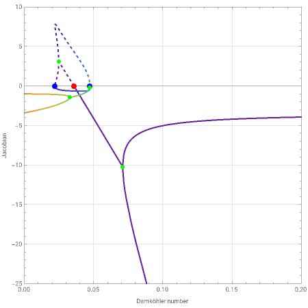
This Demonstration plots the locus of reactor steady states (concentration and temperature) versus the Damköhler number when there is multiplicity for user set values of parameters , , and =7. The unstable steady states are denoted by the dashed region of the locus. The blue dots denote the values of at the turning points, a red dot denotes the value of at a Hopf bifurcation, and the green dots denote the values where two real eigenvalues change into a complex conjugate pair.
B
β
x
2c
D
a
D
a
D
a
Time series plots for normalized concentration (in blue) and normalized temperature (in magenta) for a given set of initial conditions ( and ) and parameters are given. One can investigate the basin of attraction for the steady states. The approach to the steady state may be monotonic or oscillatory depending on the associated eigenvalues for that steady state. Initial conditions near the Hopf point are attracted to a stable periodic solution.
x
10
x
20
Details
Details
Homotopy method using arc length
Consider a set of nonlinear algebraic equations that depend on a parameter . In vector notation, these equations are represented as
N
α
f(u,α)=0
where the components of the vectors and are
f
u
f={,…,}
f
1
f
N
u={,…,}
u
1
u
N
Suppose we have found a solution to equation (5), say by Newton's method for . We represent the solution as , so that .
α=
α
0
u
0
f(,)=0
u
0
α
0
We assume that the solution is an analytic function of , that is, is continuous and differentiable. Then, given a solution , we can find a neighboring solution on the solution curve by constructing a Taylor series expansion about . If the solution curve is a multivalued function of , it is convenient to parameterize the solution in terms of a suitable parameter along the solution curve. The preferred parameter in this study is the arc length along the solution curve so that we can write equation (5) as .
u
α
u(α)
u
0
u
u
0
α
s
f(u(s),α(s))=0
The total derivative of along the solution curve is then:
f
f
s
f
u
u
s
f
α
α
s
which is a set of equations in unknowns, where the unknowns are
N
N+1
,,…,,
d
u
1
ds
d
u
2
ds
d
u
N
ds
dα
ds
Recall that (u,α)≡J(u,α) is the familiar Jacobian used in Newton's method. It is convenient to write equation (6) in matrix notation
f
u
[J⋮]
=0
f
α
u' |
α' |
where and . Thus the vector
u'≡du/ds
α'≡dα/ds
t=
u' |
α' |
is tangent to the solution curve .
u(α)
The homogeneous system of equations given by equation (7) is an underdetermined system of equations and will have a nontrivial solution if the rank of has full row rank, namely . The nontrivial solution is not unique, however. In order to obtain a unique solution, we need to add an additional equation to equation (7). The appropriate equation is given by the definition of arc length:
r
[J⋮]
f
α
r=N
u
s
u
s
2
α
s
Equations (7) and (8) represent equations in terms of the unknowns. Although equation (7) is linear in the unknowns, equation (8) is not. Moreover, the coefficient matrix in equation (7) depends on and , usually in a nonlinear way, which means that we need to solve equations (7) and (8) using an appropriate ODE solver. Matters are complicated further by the fact that is singular at bifurcation and turning points. However, the augmented matrix has full rank at turning points. This feature allows us to devise a numerical algorithm that can integrate through turning points.
N+1
N+1
u
α
J(u,α)
[J⋮]
f
α
Generally one is not really interested in how and depend on , and thus equation (8) is not really needed. The homogeneous system of equations defined by equation (7) can be solved using Cramer's rule. Thus if we define , then the vector obeys the system of equations:
u
α
s
z={,…,,α}
u
1
u
N
z
z
i
ξ
i
(-1)
det[J⋮]
f
α
-1
where is the matrix with the column removed. In the homotopy literature, Garcia and Zangwill[3] call equation (9) the basic differential equation. The advantage of using it instead of the full system of equations (7) and (8) is that equation (9) is linear in the derivatives. Note that the independent variable is not the arc length along the solution curve, but is related to arc length by
det[J⋮]
f
α
-1
th
i
ξ
s
ξ
2
z
1
ξ
2
z
2
ξ
2
z
3
ξ
Hence once the solution has been found, a simple integration gives the dependence of on . The right-hand side of equation (9) can be determined readily when is not too large using Mathematica as shown in the recent paper by Higgins and Binous[2].
z(ξ)
s
ξ
N
References
References
[1] A. Uppal, W. H. Ray, and A. B. Poore, "On the Dynamic Behavior of Continuous Strirred Tank Reactors," Chemical Engineering Science, 29(4), 1974 pp. 967–985.
[2] B. G. Higgins and H. Binous, "A Simple Method for Tracking Turning Points in Parameter Space," Journal of Chemical Engineering of Japan, 43(12), 2010 pp. 1035–1042.
[3] C. B. Garcia and W. I. Zangwill, Pathways to Solutions, Fixed Points, and Equilibria, Englewood Cliffs, NJ: Prentice–Hall, 1981.
Permanent Citation
Permanent Citation
Housam Binous, Brian G. Higgins
"Continuously Stirred Tank Reactor Using Arc-Length Parameter"
http://demonstrations.wolfram.com/ContinuouslyStirredTankReactorUsingArcLengthParameter/
Wolfram Demonstrations Project
Published: April 8, 2011