Liquid-Liquid Phase Split Calculations for Pentanary System
Housam Binous
Liquid-Liquid Phase Split Calculations for Pentanary System
Housam Binous
Housam Binous
This notebook performs liquid-liquid phase-split (flash) calculations for the pentanary system n‑Hexane(1) + n‑Octane(2) + Benzene(3) + Toluene(4) + Sulfolane(5) at 298.15 K, based on Chen et al. (Ref. 1). It defines the NRTL τ_ij parameter matrix (from the paper’s Table 6, divided by T to make it dimensionless), the nonrandomness factors are set equal to 0.2, and a generalized gamma function implementing the multicomponent NRTL activity-coefficient equation for all five components.
Two core functions are built: TPD[w1,w2,w3,w4], which evaluates the tangent-plane-distance stability criterion for a trial phase composition against the overall feed z (used to test whether the single liquid phase is unstable and to generate an initial guess for phase splitting), and eqns[...], which sets up the full nine-equation system (four isoactivity conditions, four mass-balance relations, and one Rachford–Rice-type residual) needed to solve for the two coexisting phase compositions and the phase-split fraction β.
Tie-Line Validation Loop: the notebook then applies this machinery to all four experimental tie lines from Table 7 of the paper, one at a time (“Tie line 1” through “Tie line 4”). For each, the experimental phase compositions (xPhaseI, xPhaseII) are entered, the feed z is computed as their midpoint, NMinimize performs the TPD stability test, and FindRoot solves the flash equations using the experimental compositions as the initial guess — followed by a FindMinimum cross-check on the sum of squared residuals to confirm convergence.
In every case the residual sum-of-squares converges to a vanishingly small value (10⁻⁹ to 10⁻¹³), and the recovered phase compositions and β values closely match the calculated (xcal) entries reported in the paper’s Table 7, confirming that the implemented NRTL model with the Table 6 parameters correctly reproduces the published predictions for this five-component LLE system.
Reference:
[1] J. Chen, L.-P. Duan, J.-G. Mi, W.-Y. Fei, Z.-C. Li, “Liquid–liquid equilibria of multi-component systems including n-hexane, n-octane, benzene, toluene, xylene and sulfolane at 298.15 K and atmospheric pressure,” Fluid Phase Equilibria, Vol. 173, 2000, pp. 109–119. DOI/PII: S0378-3812(00)00398-8
In[]:=
(*NRTLmodelforn-Hexane(1)+n-Octane(2)+Benzene(3)+Toluene(4)+Sulfolane(5)*)(*ParametersfromTable6,Chenetal.,FluidPhaseEquilibria173(2000)109-119*)T=298.15;(*tau_ijasgiveninTable6(units:K),dividedbyTtomakedimensionless*)tau={{0.0000,0.0000,0.1523*10^1,0.3470*10^3,0.2045*10^4},{0.0000,0.0000,-0.1635*10^3,0.1155*10^3,0.2235*10^4},{0.9089*10^2,0.2837*10^3,0.0000,0.0000,0.4032*10^3},{-0.2676*10^3,-0.8422*10^2,0.0000,0.0000,0.5623*10^3},{0.8706*10^3,0.1231*10^4,-0.1038*10^3,-0.5359*10^2,0.0000}}/T;
In[]:=
tau//TableForm
Out[]//TableForm=
0. | 0. | 0.00510817 | 1.16384 | 6.85896 |
0. | 0. | -0.548382 | 0.387389 | 7.49623 |
0.304847 | 0.951534 | 0. | 0. | 1.35234 |
-0.897535 | -0.282475 | 0. | 0. | 1.88596 |
2.92001 | 4.12879 | -0.348147 | -0.179742 | 0. |
In[]:=
(*---G[i,j]asafunctionoftemperatureT---*)G[i_,j_,T_]:=Exp[-0.2*tau[[i,j]]](*tau[i,i]=0andG[i,i]=1byconvention*)G[i_,i_,T_]:=1(*NRTLactivitycoefficient(Eq.2inthepaper),generalizedton=5components*)lnGamma[i_,x_List,T_]:=Module[{n=Length[x]},Sum[tau[[j,i]]*G[j,i,T]*x[[j]],{j,n}]/Sum[G[k,i,T]*x[[k]],{k,n}]+Sum[(G[i,j,T]*x[[j]])/Sum[G[k,j,T]*x[[k]],{k,n}]*(tau[[i,j]]-Sum[tau[[l,j]]*G[l,j,T]*x[[l]],{l,n}]/Sum[G[k,j,T]*x[[k]],{k,n}]),{j,n}]]gamma[i_,x_List,T_]:=Exp[lnGamma[i,x,T]]
In[]:=
(*TPDfunctionforstability/phase-splittesting(5components->4freevars)*)Clear[TPD];TPD[w1_?NumericQ,w2_?NumericQ,w3_?NumericQ,w4_?NumericQ]:=Module[{w5,w,gammaW},w5=1-w1-w2-w3-w4;If[w1<=0||w2<=0||w3<=0||w4<=0||w5<=0,Return[10^10]];w={w1,w2,w3,w4,w5};gammaW=Table[gamma[i,w,T],{i,1,5}];Sum[w[[i]]*(Log[w[[i]]*gammaW[[i]]]-Log[z[[i]]*gamma[i,z,T]]),{i,1,5}]](*Two-phaseisoactivity+massbalancesystem(5components)*)(*xa=aliphatichydrocarbon-richphase,xb=sulfolane-richphase*)ClearAll[eqns,z];eqns[xa1_,xa2_,xa3_,xa4_,xb1_,xb2_,xb3_,xb4_,beta_]:=Module[{xa5,xb5,xa,xb,ga,gb,K,rr},xa5=1-xa1-xa2-xa3-xa4;xb5=1-xb1-xb2-xb3-xb4;xa={xa1,xa2,xa3,xa4,xa5};xb={xb1,xb2,xb3,xb4,xb5};ga=Table[gamma[i,xa,T],{i,1,5}];gb=Table[gamma[i,xb,T],{i,1,5}];K=ga/gb;rr=Sum[z[[i]]*(K[[i]]-1)/(1+beta*(K[[i]]-1)),{i,1,5}];{xa[[1]]*ga[[1]]-xb[[1]]*gb[[1]],xa[[2]]*ga[[2]]-xb[[2]]*gb[[2]],xa[[3]]*ga[[3]]-xb[[3]]*gb[[3]],xa[[4]]*ga[[4]]-xb[[4]]*gb[[4]],xa[[1]]-z[[1]]/(1+beta*(K[[1]]-1)),xa[[2]]-z[[2]]/(1+beta*(K[[2]]-1)),xa[[3]]-z[[3]]/(1+beta*(K[[3]]-1)),xa[[4]]-z[[4]]/(1+beta*(K[[4]]-1)),rr}]
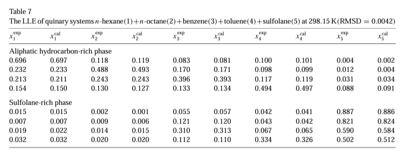
Tie line 1 from Table 7
In[]:=
(*Exampletie-linefromTable7,row1(RMSD=0.0042):n-Hexane(1)+n-Octane(2)+Benzene(3)+Toluene(4)+Sulfolane(5)*)xPhaseI={0.696,0.118,0.083,0.100,0.004};(*aliphatic-richphase,exp*)xPhaseII={0.015,0.002,0.055,0.042,0.887};(*sulfolane-richphase,exp*)z=(xPhaseI+xPhaseII)/2;z=z/Total@zTotal[z]
Out[]=
{0.355145,0.0599401,0.0689311,0.0709291,0.445055}
Out[]=
1.
In[]:=
(*TPDminimizationtofindatrialcomposition(stabilitytest)*)sol=NMinimize[{TPD[w1,w2,w3,w4],w1>=10^-6,w2>=10^-6,w3>=10^-6,w4>=10^-6,1-w1-w2-w3-w4>=10^-6},{w1,w2,w3,w4},Method->{"DifferentialEvolution"}];TPDmin=sol[[1]];Print[" TPDmin = ",NumberForm[TPDmin,{12,8}]]
TPDmin = -0.58963288
In[]:=
sol
Out[]=
{-0.589633,{w10.792708,w20.164768,w30.0194818,w40.0227932}}
In[]:=
betaGuess=0.5;
In[]:=
xaGuess={w1,w2,w3,w4}/.sol[[2]];(*fromTPD*)(*backoutxafrommassbalanceusingnormalizedz*)xbGuess=(z[[1;;4]]-(1-betaGuess)*xaGuess)/betaGuess;
In[]:=
xbGuess
Out[]=
{-0.0824181,-0.0448878,0.11838,0.119065}
In[]:=
xaGuess
Out[]=
{0.792708,0.164768,0.0194818,0.0227932}
In[]:=
(*Solveusingexperimentaltie-lineasinitialguess(recommendedforreliability)*)solRoot=FindRoot[eqns[xa1,xa2,xa3,xa4,xb1,xb2,xb3,xb4,beta],{{xa1,xaGuess[[1]]},{xa2,xaGuess[[2]]},{xa3,xaGuess[[3]]},{xa4,xaGuess[[4]]},{xb1,xbGuess[[1]]},{xb2,xbGuess[[2]]},{xb3,xbGuess[[3]]},{xb4,xbGuess[[4]]},{beta,betaGuess}},MaxIterations->1000,AccuracyGoal->10,PrecisionGoal->10]
Out[]=
{xa10.697384,xa20.119168,xa30.0808186,xa40.100453,xb10.0147222,xb20.00102687,xb30.0571066,xb40.0415624,beta0.501331}
In[]:=
(*Cross-checkviaFindMinimumonsum-of-squaresofresiduals*)FindMinimum[Sum[eqns[xa1,xa2,xa3,xa4,xb1,xb2,xb3,xb4,beta][[i]]^2,{i,1,9}],{{xa1,xaGuess[[1]]},{xa2,xaGuess[[2]]},{xa3,xaGuess[[3]]},{xa4,xaGuess[[4]]},{xb1,xbGuess[[1]]},{xb2,xbGuess[[2]]},{xb3,xbGuess[[3]]},{xb4,xbGuess[[4]]},{beta,betaGuess}},MaxIterations->10000,AccuracyGoal->10,PrecisionGoal->10]
Out[]=
{2.05112×,{xa10.697384,xa20.119168,xa30.0808186,xa40.100453,xb10.0147222,xb20.00102687,xb30.0571066,xb40.0415624,beta0.501331}}
-31
10
In[]:=
(*Recoverfullcompositionsincluding5thcomponent(sulfolane)*)xaSol={xa1,xa2,xa3,xa4,1-xa1-xa2-xa3-xa4}/.solRoot;xbSol={xb1,xb2,xb3,xb4,1-xb1-xb2-xb3-xb4}/.solRoot;betaSol=beta/.solRoot;Print["Aliphatic-rich phase (calc): ",xaSol];Print["Sulfolane-rich phase (calc): ",xbSol];Print["Phase split fraction beta: ",betaSol];
Aliphatic-rich phase (calc): {0.697384,0.119168,0.0808186,0.100453,0.00217673}
Sulfolane-rich phase (calc): {0.0147222,0.00102687,0.0571066,0.0415624,0.885582}
Phase split fraction beta: 0.501331
Tie line 2 from Table 7
Tie line 3 from Table 7
Tie line 4 from Table 7