Coupled harmonic oscillators are one of the most important models in classical mechanics, appearing in places such as molecular vibrations and circuit boards. While standard experiments show normal modes and beating phenomena, an important question still remains: how should system parameters be chosen to achieve the fastest possible energy transfer? This project finds an exact expression for the time of complete energy transfer, treating coupling strength and mass ratio as optimization variables. Starting from Newton’s laws and rewriting the systems in matrix form, I used eigenvalue analysis to find the exact normal mode frequencies. Then, by using calculus, I found out that there was a monotonic relationship between coupling strength and transfer time, with stronger coupling creating faster energy exchange. The asymmetric mass case results in a really cool finding: equal masses lead to minimal frequency splitting and the slowest transfer, whereas increasing mass asymmetry makes the frequency separation larger and accelerates energy exchange.
1. Introduction
1. Introduction
A single oscillator by itself is a complex system. But physics is never about single systems. The most realistic oscillating system is one where oscillators are coupled, in which the motion of one oscillator affects another, and where energy oscillates between them in ways that depend on the system’s design.
The two-oscillator system is the simplest example of this kind of situation. There are a lot of basics that are covered about the two-oscillator system, such as normal modes and eigenfrequencies, but the optimization problem is rarely considered. If the aim is to move energy from one mass to the other as quickly as possible, what should the coupling strength be? The mass ratio? The form of the constraints to ensure that the problem is well-posed?
These are the questions that I will answer.
2. The Single Oscillator: Foundations
2. The Single Oscillator: Foundations
Before we can discuss coupling, we need to know what we are coupling. A mass m on a spring of constant k obeys the equation of motion mẍ + kx = 0. We solve this equation symbolically, leaving parameters as symbols to ensure clean output:
In[]:=
ClearAll[x, t, A, k, m, kc]DSolve[x''[t] + x[t] == 0, x[t], t]
Out[]=
{{x[t]Cos[t]+Sin[t]}}
1
2
The solution is a sinusoid with angular frequency ω = sqrt(k/m). For k = m = 1 and initial conditions x(0) = 1, ẋ(0) = 0, the solution is simply cos(t). The total mechanical energy oscillates between kinetic and potential forms while the sum remains constant:
xsingle[t_] := Cos[t];KEsingle[t_] := (1/2) xsingle'[t]^2;PEsingle[t_] := (1/2) xsingle[t]^2;Plot{KEsingle[t], PEsingle[t], KEsingle[t] + PEsingle[t]}, {t, 0, 4 Pi},
Out[]=
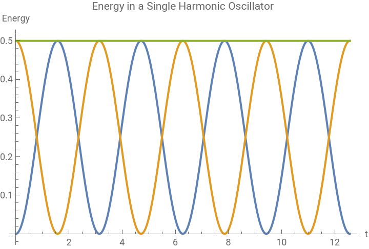


Phase space trajectories are closed ellipses, which geometrically show the basics of energy conservation. This, however, will be completely different when a second oscillator is added.
3. Formulating the Coupled System
3. Formulating the Coupled System
3.1 Physical Setup
3.1 Physical Setup
Two identical masses m are each coupled to a wall by a spring of constant k, and to each other by a coupling spring of constant k_c. The displacement x₁(t) and x₂(t) are measured from each mass’s equilibrium position.
The restoring force on mass 1 comes from two sources. One of them is its own wall spring, and the other is the coupling spring, which either stretches or compresses depending on the relative displacement of the two masses. Writing out Newton’s second law for each mass and collecting terms, the system becomes symmetric where each mass sees the same total effective spring constant (k + kc), with an off-diagonal coupling term -kc linking the two.
3.2 Matrix Representation
3.2 Matrix Representation
The two equations of motion can be combined into a single matrix equation ẍ = −Ax, where the matrix A contains all the spring constants. Setting k = 1, kc = 1/2, m = 1, we get:
In[]:=
k = 1; kc = 0.5; m = 1;A = (1/m)*{{k + kc, -kc}, {-kc, k + kc}};MatrixForm[A]
Out[]//MatrixForm=
1.5 | -0.5 |
-0.5 | 1.5 |
The diagonal elements represent each mass’s total restoring spring constant. The off-diagonal elements, both that are -kc/m, represent the coupling. They are equal because the system is symmetric if there is a swap of the two masses.
4. Eigenvalue Analysis and Normal Modes
4. Eigenvalue Analysis and Normal Modes
4.1 Finding the Eigenfrequencies
4.1 Finding the Eigenfrequencies
The problem is broken down into finding the eigenvalues of the matrix A by substituting a solution x(t) = v e^{iωt}. The characteristic equation det(A - λI) = 0 factors neatly because of the symmetric form of the matrix A:
In[]:=
ClearAll[k, kc, m, A, vals, vecs]k = 1; kc = 1/2; m = 1;A = {{(k + kc)/m, -kc/m}, {-kc/m, (k + kc)/m}};{vals, vecs} = Eigensystem[A];valsvecs
Out[]=
{2,1}
Out[]=
{{-1,1},{1,1}}
The two eigenvalues are directly related to the squared normal mode frequencies. The in-phase mode, where both masses move in unison, has the lower frequency ω₁ = sqrt(k/m), while the spring connecting the two masses neither stretches nor compresses, so it doesn’t enter the calculation. The out-of-phase mode, where the masses move in opposition, has the higher frequency ω₂ = sqrt((k + 2kc)/m).
In[]:=
ω1 = Sqrt[k/m];ω2 = Sqrt[(k + 2kc)/m];{ω1, ω2}
Out[]=
1,
2
4.2 Visualizing the Normal Modes
4.2 Visualizing the Normal Modes
The eigenvectors represent a collective motion. Comparing the two modes side by side makes it clear what each mode represents: in the first mode, the masses move in unison, and in the second mode, they push each other away:

5. The General Solution and Beating
5. The General Solution and Beating
5.1 Superposition with Localized Initial Conditions
5.1 Superposition with Localized Initial Conditions
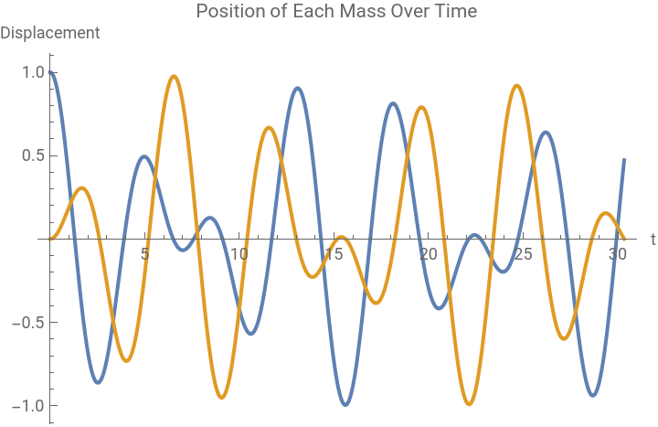
The general solution is a superposition of both normal modes. With all initial energy localized in mass 1, and x₁(0) = 1, x₂(0) = 0 so both velocities zero, the solution can be written down in terms of the normal mode amplitudes. Rather than solving with DSolve, which gives messy complex solutions for numeric parameters, we solve with the exact solution that we get from the eigenmode decomposition:
x1sol[t_] := Cos[((ω1 + ω2)/2) t] Cos[((ω2 - ω1)/2) t];x2sol[t_] := Sin[((ω1 + ω2)/2) t] Sin[((ω2 - ω1)/2) t];Plot{x1sol[t], x2sol[t]},{t, 0, 4 Pi/(ω2 - ω1)},
Out[]=
5.2 The Envelope Structure
5.2 The Envelope Structure
The solution for x₁(t) is an oscillation at the mean frequency, multiplied by an envelope that varies slowly. This is the math of the same pattern that causes two nearly equal guitar strings to sound like a single note that pulses in and out:
Δω = ω2 - ω1;Plot{Cos[(ω1+ω2)/2 * t] * Cos[Δω/2 * t], Cos[Δω/2 * t], -Cos[Δω/2 * t]},{t, 0, 4π/Δω},
Out[]=
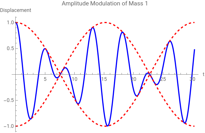


The energy in each mass varies as the square of the envelope. This oscillates at the full frequency Δω, twice as fast as the envelope variation, and the energy pumped into mass 2 is precisely the complement of the energy left in mass 1.
6. The Energy Transfer Time
6. The Energy Transfer Time
6.1 Deriving the Transfer Formula
6.1 Deriving the Transfer Formula
The energy transfer is complete when the envelope of x₁(t) first reaches zero, that is, when cos(Δω τ / 2) = 0. We solve the equation for τ without using Solve, which gives us complicated trig equations:
In[]:=
ClearAll[τ]Δωsym = Sqrt[2] - 1;τexact = Pi / Δωsym // Simplify
Out[]=
(1+
2
)πSubstituting the eigenfrequencies makes the dependence on system parameters clear:
In[]:=
τ[k_, kc_, m_] := π / (Sqrt[(k + 2kc)/m] - Sqrt[k/m])
This is the result. The energy transfer time depends only on the frequency splitting, and not on the frequencies themselves. A system with separated normal modes will transfer energy faster than a system with closely spaced modes, regardless of how fast the modes oscillate.
6.2 Verifying with Simulation
6.2 Verifying with Simulation
Before trying to optimize, we can check this formula against a direct simulation:
k = 1; kc = 0.5; m = 1;τanalytic = τ[k, kc, m];numsol = NDSolve[ {x1''[t] == -(k+kc)/m*x1[t] + kc/m*x2[t], x2''[t] == kc/m*x1[t] - (k+kc)/m*x2[t], x1[0] == 1, x2[0] == 0, x1'[0] == 0, x2'[0] == 0}, {x1[t], x2[t]}, {t, 0, 2τanalytic}];PlotEvaluate[{x1[t]^2, x2[t]^2} /. numsol],{t, 0, 2τanalytic},
The prediction matches the simulation exactly, as expected from the exact, closed solution.
7. Optimization of Coupling Strength
7. Optimization of Coupling Strength
7.1 Monotonic Behavior
7.1 Monotonic Behavior
With the transfer time formula at hand, the optimization problem can now be stated: For a given k and m, what is the optimal k_c to minimize τ? Taking the derivative with respect to k_c:
Each term in the denominator is positive for k_c > 0, so the derivative is negative for all k_c > 0. The transfer time is a monotonically decreasing function of coupling strength. There is no internal minimum without further constraints.
7.2 Constrained Optimization
7.2 Constrained Optimization
The unconstrained problem has no finite minimum, but there is a nontrivial physical constraint: fix the total stiffness K_total = k + k_c. Substituting k = K_total - k_c into the transfer time formula:
The transfer time is a monotonically decreasing function of the fraction of the total stiffness budget spent on coupling. The best possible policy is to use as much of the coupling strength budget as possible.
8. Asymmetric Mass Extension
8. Asymmetric Mass Extension
8.1 The General Eigenvalue Problem
8.1 The General Eigenvalue Problem
When m₁ ≠ m₂, the dynamical matrix is no longer symmetric in the same way, and the eigenfrequencies take a more complex form. The characteristic equation is a quadratic in ω²:
The corresponding normal mode frequencies are the square roots of these eigenvalues. The two frequencies are no longer symmetric around a simple midpoint, and the beating pattern is more complicated.
The general formula for the two frequencies involves a square root of a discriminant that measures how asymmetric the system is:
8.2 Optimizing the Mass Ratio
8.2 Optimizing the Mass Ratio
For fixed total mass M = m₁ + m₂ and fixed spring constants, we ask how mass distribution affects frequency splitting. We define the splitting as a function of m₁ directly from the mass-weighted eigenvalue calculation:
The graph shows a U-shape with a minimum at m₁ = 1. Equal masses produce the smallest frequency gap between normal modes and therefore the slowest energy transfer. Asymmetric distributions increase the splitting, where a very unequal pair like m₁ = 0.2, m₂ = 1.8 transfers energy roughly three times faster than the equal-mass case.
To make the relationship between mass distribution and transfer speed accurate, the table below samples five points across the domain. The splitting Δω is read from the mass-weighted eigenvalue calculation, and τ = π/Δω gives the time for complete energy transfer. Notice that the table is symmetric around m₁ = 1, reflecting the physical symmetry of the system under relabeling of the two masses. The equal-mass row has the largest τ, confirming it is the slowest configuration.
9. Dimensional Analysis and Scaling
9. Dimensional Analysis and Scaling
Removing units helps to focus on the physically significant combinations of parameters. The intrinsic time scale of the problem is the period of the decoupled oscillator, T₀ = 2πsqrt(m/k). Scaling the transfer time in units of T₀ and introducing the dimensionless coupling α = kc/k:
In the strongly coupled regime for α ≫ 1, the transfer time is proportional to 1/sqrt(k_c), because the leading term in the denominator is proportional to sqrt(2k_c/m). The scaling rule has a very clear physical interpretation: increasing the coupling strength by a factor of two will shorten the transfer time by a factor of sqrt2, with diminishinng returns for large coupling.
10. Visualization and Phase Space
10. Visualization and Phase Space
The complete process of energy transfer is represented in a phase space animation. The path of mass 1 in the (x₁, ẋ₁) plane is an ellipse whose scale shrinks to zero as energy is transferred away, then expands back as energy is transferred back. Based on the numerically solved solution in Section 6:
The moment of complete energy transfer can be seen as the trajectory collapses toward the origin and mass 1 is momentarily near rest at its equilibrium. The trajectory then re-expand as energy returns.
11. Discussion
11. Discussion
The methods that I used, such as, eigenvalue decomposition, calculus, and extremization, each work together in a sense. The eigenvalues of the coupling matrix directly finds a closed-form transfer time. That transfer time is a monotone function of coupling strength in both the unconstrained and stiffness-constrained cases, where stronger coupling always wins. The extension to asymmetric masses shows a counterintuitive result, in which equal mass is actually the worst configuration for transfer speed under fixed total mass. When masses are unequal, one natural frequency is high and the other low, spreading the normal modes further apart and accelerating energy exchange.
The result is that energy transfer rate is determined by frequency splitting, not by the individual frequencies. While this is not immediately understandable from the optimization work, an important part that can be found is that in order to transfer energy efficiently, the separation between the system’s normal modes should be maximized. This can be done, depending on the constraints, by adjusting the coupling constant, matching the masses, or distributing the stiffness.
12. Conclusion
12. Conclusion
This analysis found an exact expression for the complete energy transfer time between coupled harmonic oscillators and optimized it. Transfer time basically depends only on the splitting between normal mode frequencies, and it decreases monotonically with coupling strength in both the unconstrained and constrained cases; no interior optimum exists, and maximum coupling always minimizes transfer time. The asymmetric mass extension shows that equal mass distribution minimizes frequency splitting and produces the slowest energy transfer for a given total mass. Asymmetric configurations, where one mass is much heavier than the other, maximize the frequency gap and minimize transfer time. Together, these results find a feasible way to predict and optimize how energy moves between oscillators.
CITE THIS NOTEBOOK
CITE THIS NOTEBOOK
Optimization of energy transfer in coupled harmonic oscillators
by Pavel Pomozov
Wolfram Community, STAFF PICKS, June 14, 2026
https://community.wolfram.com/groups/-/m/t/3732981
by Pavel Pomozov
Wolfram Community, STAFF PICKS, June 14, 2026
https://community.wolfram.com/groups/-/m/t/3732981