Goal: Our study focuses on exploring GPT-2’s capabilities in detecting and understanding contexts in text. We aim to determine whether context learning occurs gradually or if different components in GPT-2 are responsible for distinct context extraction. By delving into the inner workings of GPT-2, we aim to gain a better understanding of its ability to distinguish contexts.
Result: Through our probing technique, we have gained valuable insights into the context detection capabilities of GPT-2. Through numerical investigation, we have discovered that certain self-attention layers are likely responsible for specific types of context detection. Furthermore, we have observed that context detection occurs both gradually and abruptly within GPT-2. While the overall quality of the input signal tends to improve as it traverses the layers, there are notable instances where sudden jumps occur, with the pattern influenced by the specific context being analyzed.
Future Work: To obtain a comprehensive understanding of GPT-2’s inner workings, further exploration is needed. This includes studying each attention head independently, meticulously examining and fine-tuning the probe’s design, and conducting investigations on larger datasets to uncover the diverse roles of GPT-2’s components. Additionally, the exploration of opposing sentences, differing by only a single word yet yielding distinct contexts, holds promise in unraveling the intricate circuits of GPT-2.
Disclaimer: The views expressed in this statement represent the author’s personal opinion and understanding. The author recognizes that a two-week timeframe may not allow for extensive language learning or thorough research to ascertain the uniqueness of an idea. It is also acknowledged that the initial search conducted might not have encompassed all possibilities, leaving room for the existence of similar approaches or perspectives beyond the limited scope of the search.
Over the past few years, Transformer-based language models have gained considerable recognition for their exceptional accomplishments. One notable milestone was the emergence of GPT-2 in 2019, marking the arrival of a model that could generate text with an uncanny resemblance to human language. Nevertheless, to ensure the responsible and effective application of these models in real-world situations, it remains crucial to develop a profound comprehension of their underlying behaviors.
In this note, we embark on an exploratory journey into the depths of GPT-2, delving into its inner workings and examining the outputs of various layers. We kick things off by providing an overview of GPT-2’s structure and shedding light on the intricate computations performed on input strings. Drawing inspiration from electrical circuits, we devise a probe to gain insights into the internal mechanisms of GPT-2. We fine-tune our probe and delve into the specifics of our approach. Armed with this probing technique, we apply it to different datasets, meticulously tracing the signal path from the input port to the output port. Our findings are then meticulously dissected, and we also outline potential avenues for future exploration.
In this note, we embark on an exploratory journey into the depths of GPT-2, delving into its inner workings and examining the outputs of various layers. We kick things off by providing an overview of GPT-2’s structure and shedding light on the intricate computations performed on input strings. Drawing inspiration from electrical circuits, we devise a probe to gain insights into the internal mechanisms of GPT-2. We fine-tune our probe and delve into the specifics of our approach. Armed with this probing technique, we apply it to different datasets, meticulously tracing the signal path from the input port to the output port. Our findings are then meticulously dissected, and we also outline potential avenues for future exploration.
Exploring the inner structure of GPT-2
Exploring the inner structure of GPT-2
GPT-2 employs a multi-layer Transformer architecture that operates on a sequence of “tokens” as input. It processes the input through various layers, including an embedding layer, multiple transformer decoder layers, and an output layer.
In[]:=
gpt2LanguageModel=NetModel["GPT2 Transformer Trained on WebText Data","Task"->"LanguageModeling"];Information[gpt2LanguageModel,"SummaryGraphic"]
Out[]=

Before delving into the intricacies of these layers, let us first discuss how the input string turns into tokens. GPT-2 utilizes a byte-level BPE (Byte Pair Encoding) tokenizer, which breaks down the input string into a series of sub-word tokens. These sub-word tokens do not directly correspond to individual words but rather represent smaller units of text. The number of tokens used in GPT-2’s vocabulary is 50,257. These tokens allow GPT-2 to effectively process and generate text.
In[]:=
tokenizerBPE=NetExtract[gpt2LanguageModel,"Input"];
To illustrate the tokenizer’s functionality, let’s consider the sentence “I am writing a report about GPT-2.”. We will now proceed to parse this sentence using the tokenizer.
In[]:=
tokenizedInput=tokenizerBPE["I am writing a report about GPT-2."];Print["The output of the tokenizer:",tokenizedInput]
The output of the tokenizer:{50217,461,3342,2,734,291,147,11316,50245,50240,50244}
Upon tokenizing the input string using a tokenizer, the tokens can be transformed back into the original sentence by applying the inverse process of the tokenizer. Similarly, at the output stage of GPT-2 for generating the next token, the model converts a unit vector of size 50,257 into a token. By reversing the tokenization process, we are able to retrieve the original sequence in its entirety.
In[]:=
tokenizerReverseBPE=NetExtract[gpt2LanguageModel,"Output"][UnitVector[50257,#]]&;Print["reversing the tokenization process returns:",tokenizerReverseBPE/@tokenizedInput]
reversing the tokenization process returns:{I, am, writing, a, report, about, G,PT,-,2,.}
As evident from the example, the string “ GPT-2” has been tokenized into sub-word tokens: “ G”, “PT”, “-”, “2”. Now, let’s explore the computations performed on {50217, 461, 3342, 2, 734, 291, 147, 11316, 50245, 50240, 50244} to gain insight into the underlying structure of GPT-2.
The embedding layer
The embedding layer
Once the input sequence has been parsed and transformed into a list of integers using the tokenizer, GPT-2 proceeds to pass the resulting integers as input to the embedding layer.
In[]:=
embeddingLayer=NetRename[NetExtract[gpt2LanguageModel,1],{"posembed"->"sequence id","embeddingpos"->"position embed","embeddingtokens"->"token embed"}];Show[Information[embeddingLayer,"FullSummaryGraphic"],ImageSize->{400,100}]
Out[]=
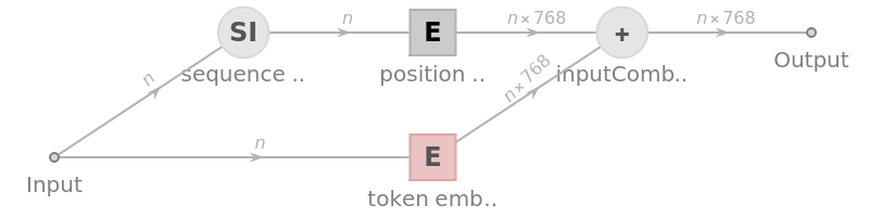
The input integers of length n (in our example, n = 11) are processed through two distinct paths: (1) the token embedding path and (2) the position embedding path.
In[]:=
tokenEmbeddingPath=NetTake[embeddingLayer,{"token embed"}];posEmbeddingPath=NetTake[embeddingLayer,{"sequence id","position embed"}];GraphicsGrid[{{Labeled[Information[tokenEmbeddingPath,"FullSummaryGraphic"],"token embedding path"],Labeled[Information[posEmbeddingPath,"FullSummaryGraphic"],"position embedding path"]}},ImageSize->Large]
Out[]=

(1) The token embedding path maps integers to a vector space of size 768. In other words, it transforms each input integer into a 768-dimensional vector. As a result, we obtain a list of n vectors, where each vector has a size of 768. In our example, this process will yield a list of 11 vectors, with each vector having a size of 768.
In[]:=
tokenEmbeddingPathInput=tokenEmbeddingPath[tokenizedInput];Print["the dimension of the output of the embedding path:",Dimensions[tokenEmbeddingPathInput]]
the dimension of the output of the embedding path:{11,768}
(2) The position embedding path captures the positional information of each token. It comprises two layers: the sequence indices layer and the position embedding layer . The sequence indices layer takes a list of integers of size n and generates a corresponding sequence of numbers {1, 2, ..., n}, disregarding the content of the input integers. This sequence is then fed into the embedding layer, which maps each integer to a 768-dimensional vector, resulting in a collection of n vectors, each with a size of 768.


In[]:=
posEmbeddingPathInput=posEmbeddingPath[tokenizedInput];Print["the dimension of the output of the position embedding path:",Dimensions[posEmbeddingPathInput]]
the dimension of the output of the position embedding path:{11,768}
Finally, the two lists of 768-dimensional vectors are combined by elementwise summation, resulting in the output of the embedding layer. This operation effectively produces a sequence that is nearly identical to what would have been obtained by directly passing the input integers through the entire embedding layer. Any differences that arise are negligible and primarily stem from implementation details.
In[]:=
embedOutput=posEmbeddingPathInput+tokenEmbeddingPathInput;Print["absolute error between direct calculation and using the net = ",Max@Abs@(embedOutput-embeddingLayer[tokenizedInput])]
absolute error between direct calculation and using the net = 2.16067×
-7
10
Throughout the remainder of the article, we treat any list of length n consisting of 768-dimensional vectors as an n × 768-dimensional matrix. In this matrix representation, the row corresponds to the element of the list. Notice that each row corresponds to an specific token.
th
k
th
k
The decoding layer
The decoding layer
The output of the embedding layer is subsequently passed through a series of 12 decoding layers and a normalization layer. In each decoding layer, an n x 768-dimensional matrix serves as the input, which undergoes computations to generate a new n x 768-dimensional matrix. These computations involve incorporating context and applying various transformations to the input matrix. The resulting matrix from each decoding layer acts as the input for the subsequent layer, creating a sequential flow of information through the decoding layers. It is within these decoding layers that the magic of GPT-2 truly unfolds.
In[]:=
decoderLayers=NetExtract[gpt2LanguageModel,"decoder"];Information[decoderLayers,"SummaryGraphic"]

Each decoder consists of two sub-layers: a self-attention layer and a feed-forward layer. The self-attention layer allows tokens within the sequence to interact and exchange contextual information. The feed-forward layer performs non-linear transformations on each token independently, further refining their features. Each layer has its own set of parameters that are learned during the training process. These parameters enable the model to capture and encode different aspects of the input sequence at each layer, allowing for increasingly complex and nuanced representations as information flows through the network.
In[]:=
selfAttention=NetRename[NetFlatten@NetExtract[decoderLayers,{"1","1"}],{"norm"->"normalization","attention/6"->"linear map","attention/5"->"attention","attention/4"->"scale","attention/3"->"value","attention/2"->"query","attention/1"->"key"}];feedForward=NetRename[NetFlatten@NetExtract[decoderLayers,{"1","2"}],{"norm"->"normalization","linear1"->"linear expand","linear2"->"linear shrink"}];GraphicsGrid[{{Labeled[Information[selfAttention,"FullSummaryGraphic"],"self-attention layer"]},{Labeled[Information[feedForward,"FullSummaryGraphic"],"feed-forward layer"]}},ImageSize->{500,470}]
Out[]=
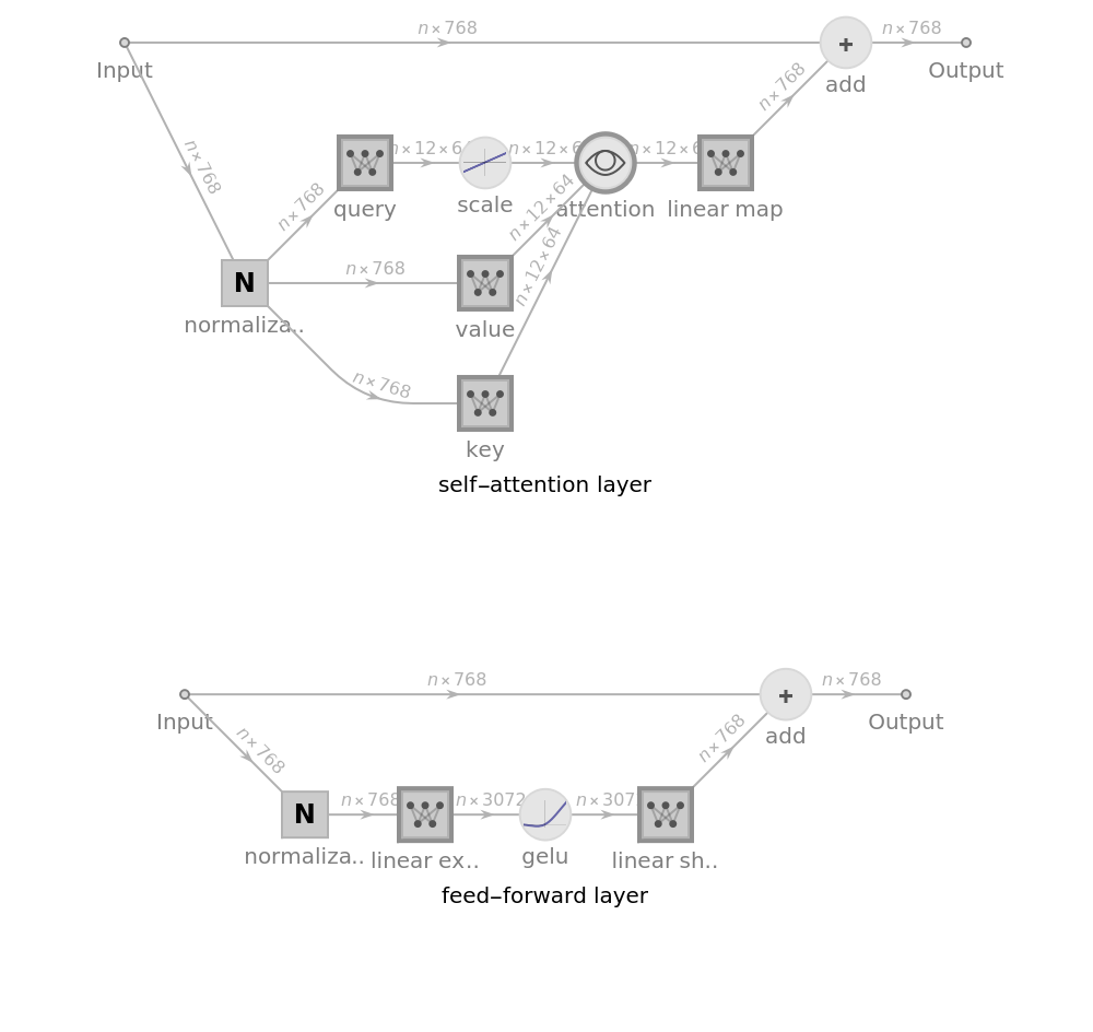
The n x 768-dimensional matrix, which serves as input to a decoder, undergoes processing through the self-attention layer. The self-attention layer calculates attention weights that represent the importance of each token’s connection with the previous tokens in the sequence. These attention weights are then used to compute a weighted sum of the values, which is subsequently added to the original input to produce the output of the self-attention layer. This mechanism allows the model to incorporate context and capture dependencies between tokens in the sequence. The self-attention layer in GPT-2 comprises various components. These include normalization, query, key, and value layers, along with scaling, attention mechanisms, and a linear transformation.
1
.The normalization layer operates independently on each row of the input matrix. Each row of the input matrix is independently normalized by subtracting the mean of that specific row and dividing it by the square root of the variance plus a small value epsilon. This normalization step ensures that each row has a mean of zero and a variance of close to one. After normalization, an element-wise scaling is applied to each row of the matrix. Additionally, a drift term is introduced, which contributes to the final output of the normalization process. Here is a concise code snippet that demonstrates the same task using the terms of the normalization layer.

In[]:=
scale=Normal@NetExtract[selfAttention,{"normalization","Scaling"}];bias=Normal@NetExtract[selfAttention,{"normalization","Biases"}];eps=Normal@NetExtract[selfAttention,{"normalization","Epsilon"}];meanTmp=Mean[Transpose[embedOutput]];varTmp=Total[Transpose[Power[(embedOutput-meanTmp),2]]]/768;normAttOutput=bias+#&/@(scale*#&/@((embedOutput-meanTmp)/Sqrt[varTmp+eps]));Print["absolute error between direct calculation and using the net = ",Max@Abs@(normAttOutput-NetExtract[selfAttention,"normalization"][embedOutput])]
absolute error between direct calculation and using the net = 7.92241×
-8
10
2
.The query layer generates query vectors. These query vectors capture specific information about the tokens and encode the questions or queries that guide the attention mechanism. To obtain these query vectors, each row of the input matrix undergoes a linear transformation, where the row is multiplied with the query matrix. Additionally, a drift term is added to the result of the multiplication. The resulting vector is then divided into 12 subvectors, each with a length of 64. These subvectors represent the query vectors for the 12 attention heads. The query vectors are subsequently used within the attention mechanism to calculate attention weights.

In[]:=
queryWeights=Normal@NetExtract[selfAttention,{"query","Net","Weights"}];queryBiases=Normal@NetExtract[selfAttention,{"query","Net","Biases"}];queryOutput=ArrayReshape[(queryBiases+queryWeights.#)&/@normAttOutput,{Length[normAttOutput],12,64}];Print["absolute error between direct calculation and using the net = ",Max@Abs@(queryOutput-NetExtract[selfAttention,"query"][normAttOutput])]
absolute error between direct calculation and using the net = 1.43023×
-6
10
3
.The scale layer scales the queries with 0.125.

In[]:=
scaleOutput=0.125*queryOutput;Print["absolute error between direct calculation and using the net = ",Max@Abs@(scaleOutput-NetExtract[selfAttention,"scale"][queryOutput])]
absolute error between direct calculation and using the net = 2.86286×
-8
10
4
.The key layer generates key vectors, which are obtained through a similar process as the query vectors; the key vectors are derived by subjecting each row of the input matrix to a linear transformation. The distinction lies in the specific parameters used for this transformation. The key vectors encodes the key aspect of each token and work in conjunction with the query vectors to calculate attention weights.
In[]:=
keyWeights=Normal@NetExtract[selfAttention,{"key","Net","Weights"}];keyBiases=Normal@NetExtract[selfAttention,{"key","Net","Biases"}];keyOutput=ArrayReshape[(keyBiases+keyWeights.#)&/@normAttOutput,{Length[normAttOutput],12,64}];Print["absolute error between direct calculation and using the net = ",Max@Abs@(keyOutput-NetExtract[selfAttention,"key"][normAttOutput])]
The output layer
The output layer
GPT-2 text generation
GPT-2 text generation
GPT-2 is a powerful language model designed to generate the next token based on a given input sequence. Let’s take an example: if we provide the input text “I am writing a report about GPT-2.”, the 10 most probable tokens that could follow are listed below:
Notice that that the 3rd element in the list above represents the next line character “\n”. After generation, this character is added to the end of the string and fed back into the GPT-2 model to generate the next character. However, this process is inefficient because the values and keys associated with the previous tokens remain unchanged. Storing the values and keys of the previous tokens across all layers can significantly reduce the usage of the computational resources. This concept is the main idea behind the gpt2TokenGenerator function, which is sourced from the Wolfram neural net repository (with added comments). This is achieved through the use of the NetUnfold function, which unfolds the attention layers and provides access to the inner states. The next 20 tokens generated by the GPT-2 for the input string “I am writing a report about GPT-2.”, are given as follows:
Now that we have covered the basics of GPT-2 (which was not that long!), it’s time to delve deeper into understanding the output of each layer.
Does GPT-2 detect and understand contexts in text?
Does GPT-2 detect and understand contexts in text?
At a high level, the depicted illustration bears resemblance to an electrical grid, where an input current (in the form of an n x 768-dimensional matrix) is processed to generate an output current (also an n x 768-dimensional matrix). Within this grid, the text context is embedded within the current signal. The question then arises: How much text context is added at each component of this grid? Drawing from the same analogy, we must develop a probing mechanism to assess the amount of context embedded within each edge of the depicted graph.
Designing a probe
Designing a probe
Designing an appropriate probe can be challenging and may require trial and error. However, due to time constraints, we will adopt a straightforward and simplified approach. Our methodology involves supplying labeled data to the computational graph and training a simple classifier to classify the output of each component. We will assess the accuracy rate of the classifier on the test data, which will serve as our
measure of context detection at each specific component. We will use the Movie Review Polarity Data at Wolfram repository to design our probe.
measure of context detection at each specific component. We will use the Movie Review Polarity Data at Wolfram repository to design our probe.
How simple is too simple?
How simple is too simple?
To probe these ports, we utilize the probeData function, which requires input parameters such as a netModel, the names of the ports to probe, the resource data, the size of the data to read from the resource, and the target device for code execution. Further information regarding this process can be found at the end of the post.
After retrieving the output from all the ports, we train a simple classifier to classify the labels, allowing us to obtain the test error and loss associated with this classifier. In order to mitigate the risk of overfitting, we employ a straightforward classifier. Nevertheless, this prompts the question: How simple is considered too simple for the classifier?
We will use a classifier structure consisting of a dropout layer at the input, followed by a linear layer and a softmax layer at the output.
Notice that the current probeData function uses a different classifier that we will discuss shortly. To regenerate the plots, here is the output if the above probe is replaced with the current classifier in the probeData function. Running the code from scratch took about 12 hours on my laptop.
Using the above result file, we demonstrate the output function by calling the displayResults function. The displayResults function takes the output of probeData as input and displays the following: a sorted dataset based on the error rate, a bar chart (which will be discussed later), and a flow graph with colored edges based on the accuracy rate (one minus the error rate).
Although the results appear promising, there is one suspicious observation after careful examination. In decoder 7, the classifier seems to struggle with classifying the input to the normalization layer. However, it performs significantly better at the output of the normalization layer. This raises doubts since normalization is a linear operation. It appears that the chosen classifier is too simplistic, to the extent that a linear transformation has significantly improved its accuracy.
The probe
The probe
To address the issue of simplicity in the previous probe, a straightforward solution is to incorporate a normalization layer into the input.
This is the structure of the probe in the probeData function. It is important to note that the output vectors of different components have varying sizes. Therefore, the code in probeData accounts for this discrepancy. Probing all ports using the above probe takes almost 24 hours.
To reproduce the same result, simply uncomment and execute the following command.
This result provides a much clearer understanding. It is worth noting that in decoder 7, there is a noticeable shift in context detection after the attention layer, which aligns with our expectations. Hence, the answer to the section’s title is a resounding ‘yes’: GPT-2, originally designed for generating the next token, does indeed exhibit context detection capabilities. Interestingly, the most remarkable context detection in the aforementioned example occurs at the output of the attention layer (distinct from the self-attention layer) in the 8th decoder, rather than at the final output. With our probe successfully designed, we will now proceed to apply it to various resource data.
Probe this, probe that!
Probe this, probe that!
With limited resources, it becomes impractical to probe all available ports. Additionally, based on the observations from the previous figure, it appears that certain components have minimal impact on altering the error rate between their input and output. Therefore, we have decided to focus our probing efforts on specific components. These components include the output of each addition layer, the output of the linear map in the self-attention layer, the output of the linear compression layer in the feed-forward layer, and the final output of the network. By targeting these components, we effectively probe a total of 50 ports.
It is important to acknowledge certain observations from the previous figure. For instance, in decoder 7, the output of the attention layer exhibits a substantial improvement in detection compared to decoder 6’s output. However, this positive impact is somewhat mitigated by the subsequent linear layer that follows the attention layer. Consequently, it might appear that the attention layer in decoder 7 plays a comparatively lesser role in context detection. Nevertheless, given our limited resources, we are compelled to make choices based on available constraints. Probing the output of the linear layers is more favorable choice since it corresponds to the signal added to the residual stream.
What each figure displays?
What each figure displays?
Each figure has 3 components:
1
.The dataset representation organizes the probing results according to the error rate.Notice that we have assigned more meaningful names to each port.
2
.The Bar charts depict the differences in accuracy rates between the input and output sections that we probe. Specifically, the Bar chart for the self-attention layer showcases the changes in accuracy rates from the input of the normalization layer to the output of the linear layer. Similarly, the Bar chart for the feed-forward layer visualizes the variations in accuracy rates within the feed forward layer. Additionally, the Bar chart for the residual attention layer highlights the accuracy rate changes between the input and output of the addition layer in the self-attention layer. Likewise, the Bar chart for the residual feed-forward layer provides insights into the comparison of accuracy rates within the feed forward layer.
3
.The flow graph visualizes accuracy rates through edge coloring, where warmer edges indicate higher accuracy rates and colder edges represent lower accuracy rates. In this representation, the color of each directed edge is determined by the accuracy rate of the source node.
Movie Review Polarity
Movie Review Polarity
The movie review polarity dataset is available through the Wolfram Data Repository. This dataset comprises 7,462 training data examples and 3,200 test data examples.
Each element within this dataset is a movie review that has been labeled as either “positive” or “negative” based on the content of the review.
Probing this data set results in the following figure.
Comment Toxicity
Comment Toxicity
The comment toxicity dataset consists of tweets that have been labeled with toxicity levels ranging from 0 to 1. This dataset is accessible online on the Kaggle website in .csv format. We have parsed and cleaned the data for our analysis. We have set the threshold at 0.5, where any comment with a toxicity level greater than 0.5 is considered toxic, while comments with a toxicity level below 0.5 are considered non-toxic. To ensure a balanced representation, we randomly sampled from the dataset while ensuring a relatively equal number of toxic and non-toxic comments in both the training set and the test set. The resulting dataset consists of 18,160 training data examples and 1,962 test data examples.
Each element within this dataset is a tweet that has been labeled as either “positive” or “negative” based on whether it is toxic or not.
Running the code took 3 hours on my laptop.
To reproduce the same result, simply uncomment and execute the following command.
Probing this data set results in the following figure .
Political News Articles
Political News Articles
The political news article is derived from an extensive online dataset on Kaggle, encompassing approximately 210,000 news headlines from 2012 to 2022 sourced from HuffPost. The original dataset is in JSON format, which cannot be directly opened using the Import function. Instead, the dataset needs to be read line by line, treating it as a stream. From this dataset, we have randomly sampled 8,000 political articles and 8,000 non-political articles. For each article, we have merged the “headline” with its corresponding “short_description”.
Each element within this dataset is a news article that has been labeled as either “positive” or “negative” based on whether it is a political news article or not.
Running the code took 3 hours on my laptop.
To reproduce the same result, simply uncomment and execute the following command.
Probing this data set results in the following figure .
Healthy Living Articles
Healthy Living Articles
This data set is also a part of the HuffPost news articles. From this dataset, we have randomly sampled 6500 articles about healthy living style and 6500 articles unrelated articles. For each article, we have merged the “headline” with its corresponding “short_description”.
Each element within this dataset is a news article that has been labeled as either “positive” or “negative” based on whether it is a healthy living style news article or not.
Running the code took 3 hours on my laptop.
To reproduce the same result, simply uncomment and execute the following command.
Probing this data set results in the following figure .
Political News Articles vs Healthy Living Articles
Political News Articles vs Healthy Living Articles
Finally, we compare political news articles with healthy living news articles. These are sampled from the same data set, by selecting 6500 random political news articles and 6500 random healthy news articles.
Each element within this dataset is a news article that has been labeled as either “positive” or “negative” based on whether it is a healthy living style news article or a political news article.
Running the code took 3 hours on my laptop.
To reproduce the same result, simply uncomment and execute the following command.
Probing this data set results in the following figure .
Discussion
Discussion
Certainly, GPT-2 exhibits the ability to differentiate between different types of input strings. Moreover, it is intriguing to observe that various modules within GPT-2 demonstrate varying performances depending on the input data. While a thorough investigation is necessary to draw precise conclusions, we will make our best effort to interpret the presented results. We most intriguing observations are highlighted in the last two bullet points.
◼
The model exhibits its weakest performance at the output of the embedding layer, which is not surprising considering that the last row of the n x 768-dimensional embedding layer output encodes only the last character of the string and its position. It is expected that the classifier’s accuracy rate when applied to this output would hover around 50%, depending on the label distribution in both the training and test datasets. However, when comparing political articles to those on healthy living styles, this accuracy rate jumps to 0.65. This can be related to the differing length distributions between these two article types.
◼
The most substantial increase in accuracy occurs at the first self-attention layer, surpassing all other layers. This finding remains consistent across different data types. However, this outcome is to be anticipated, considering that the first self-attention layer introduces contextual information into the residual stream. It further suggests that, in the initial self-attention layer, each token attends to all preceding tokens and not their immediate neighbors. We will promptly validate this hypothesis.
◼
Upon examining the bar chart, it becomes apparent that the extraction of context predominantly occurs at the self-attention layers. This observation should not be surprising, as these layers are the only ones that mixes the tokens, enabling the extraction of contextual relationships within the text.
◼
The highest accuracy rate may not necessarily occur at the output layer; instead, it can be found somewhere in between. This observation is particularly evident when analyzing movie review data.
◼
The accuracy of detection varies across different data types, with the classifier demonstrating better performance on news data. This observation holds true not only for the specific news articles discussed in this report but also for other news articles in general. A potential explanation for this discrepancy lies in the training data used for GPT-2. According to the Wolfram repository, the GPT-2 model utilized in our study was trained on the WebText dataset, which consists of web pages scraped with a focus on document quality. It is plausible that news articles were part of this dataset. Additionally, news articles are high quality documents, as opposed to rants on Twitter or movie reviews written by individuals. This may have also contributed to the classifier’s better performance.
◼
The chart associated with the attention layer exhibits distinct patterns across different data types. Notably, an intriguing pattern emerges in relation to the self-attention layer in decoder 5. In both the movie review and comment toxicity datasets, this module enhances the detection accuracy. However, for all news-related articles, the module falls short in improving the classifier’s accuracy. This observation suggests that the self-attention layer in decoder 5 excels at capturing the tone of the input string, considering that news articles often adopt a neutral tone.
◼
Another interesting observation arises when comparing the performance of different self-attention layers across news datasets and other datasets. In the case of news articles, the classifier’s performance is generally positive in the last few layers. However, for non-news articles, the performance is more unpredictable, showing sudden improvements in specific self-attention layers. This is related to the fact that GPT-2 was trained on high-quality documents. To gain deeper insights into its internal structure, a closer examination of non-news-related articles is recommended.
Thus far, our focus has been on analyzing multiple sentences collectively. However, let us now shift our attention to a specific sentence comparison. We will examine the performance of GPT-2 on the following contrasting sentences: “I am in a good mood and I want to” and “I am in a bad mood and I want to”. Despite sharing almost identical words, these sentences convey opposite tones. To gain insights, we will employ GPT-2 to generate the next 5 tokens for each of these sentences.
GPT-2 demonstrates the ability to discern the tone of these two sentences. To gain further insights, let’s closely examine the attention weights employed in generating the first token.
It is evident that each token, even in the first layer, attends to all the preceding tokens. Additionally, the attention weights of the first layer appear to be nearly identical for both sentences. However, upon closer examination of the top 15 possibilities for the next token, we observe distinct predictions.
Observe that the word “thank” has appeared in the left bar chart and not the right one. By tracing the input signal of both sentences, one can identify the point at which they begin to diverge. Exploring this idea may potentially unveil the distinctive roles played by different layers, contributing to a deeper understanding of its internal circuits.
Conclusion and future work
Conclusion and future work
Our understanding of why GPT-2 operates as it does remains limited. At a superficial level, GPT-2 functions as a computational unit that takes in an input, performs nonlinear calculations, and generates an output token. The crucial mechanisms lie within the attention layers, where each token formulates queries, scores previous tokens using their keys, and combines the weighted average of value vectors as its response. This enables the token to extract information from preceding tokens. However, the specific roles played by different layers within this process remain unclear at this stage. To gain deeper insights, it is necessary to conduct a thorough study of the attention heads within each attention layer, ideally on significantly larger datasets. However, this level of analysis surpasses the computational capacity currently available during the writing of this report. Moreover, an intriguing avenue for future research lies in investigating “opposing sentences” that differ by only one word, yet result in distinct contexts. Such an analysis holds great potential for uncovering the underlying circuits and mechanisms employed by GPT-2. At the end, I gratefully acknowledge the invaluable assistance and support provided by my mentor Christian Pasquel, Daniel Sanchez. In an ironic twist, I utilized ChatGPT to improve the writing quality of this report, leading to a situation where the “child” (ChatGPT) assisted me in describing its “parent” (GPT-2).
Initializations
Initializations
Port and connection renaming functions in GPT-2: enhancing network structure visualization
Port and connection renaming functions in GPT-2: enhancing network structure visualization
CITE THIS NOTEBOOK
CITE THIS NOTEBOOK
Unveiling the Enigma of GPT-2: Decoding its Contextual Inference Mechanism
by Mehrdad Moharrami
Wolfram Community, STAFF PICKS, July 13, 2023
https://community.wolfram.com/groups/-/m/t/2960047
by Mehrdad Moharrami
Wolfram Community, STAFF PICKS, July 13, 2023
https://community.wolfram.com/groups/-/m/t/2960047