Plotting the Spherical Heat Equation Solutions During Phase Change
Plotting the Spherical Heat Equation Solutions During Phase Change
Safi Ahmed
In this notebook, we are considering a spherical material undergoing a melting process. Heat transfer occurs from the outer surface inward, causing the solid core to shrink while the liquid phase forms around it.
This problem is inspired by the work in [1], where the authors found solutions for the temperature in both the solid and liquid regions as a spherical particle melts.
The goal of this notebook is to show how the spherical particle melts over time and to walk through the steps needed to create the plot shown in Figure 3(a) of the paper.
1. Parameters
1. Parameters
In this section, we will input the various parameters used in the equations into the code.
1.1. Physical properties of Paraffin
1.1. Physical properties of Paraffin
The phase change material used in the project is paraffin, for which we define the physical properties as follows:
In[]:=
ClearAll["Global`*"];(*Thisfunctionclearsanypastdefinitions*)
In[]:=
Tm=303;(*meltingtempreratureoftheparaffin*)ρs=880;ρl=760;ρ=ρl;(*densityatsolidandliquidstates*)ks=0.24;kl=0.15;(*thermalconductivityatsolidandliquidstates*)cps=2.4*;cpl=1.8*;(*specificheatatsolidandliquidstates*)q=179*;(*latentheatoffusion*)vd=3.42;(*dynamicviscosityofparaffin*)vk=;(*kinematicviscosityofparaffin*)
3
10
3
10
3
10
vd
ρ
1.2 . System parameters
1.2 . System parameters
Here, we define the system parameters that describe the physical setup of the melting problem:
In[]:=
keq=1;(*equivalentthermalconductivity;sinceRayleighnumber=0(i.e.≤5×)forfigure3(c),keqisassumedequalto1*)R=5*;(*radiusofthesphere*)Ti=295;(*initialtemperatureoftheparaffin*)
4
10
-2
10
1.3. Dimensionless numbers
1.3. Dimensionless numbers
Here, we define the dimensionless numbers, which include the Stefan number, Biot number, and other factors essential for scaling the problem.
In[]:=
ste=0.05;(*Stefannumber*)ra=0;(*Rayleighnumber*)bi=10;(*Biotnumber*)G=0;(*dimensionlessheatsinkparameter*)
2. Formulas for heat transfer calculations
2. Formulas for heat transfer calculations
Similar to the parameters above, here we define key dimensionless numbers and formulas that describe the heat transfer and contribute to the solutions that we will examine next.
In[]:=
αs=;(*thermaldiffusivityatsolidstate*)αl=;(*thermaldiffusivityatliquidstate*)pr=;(*Prandtlnumber*)gdot=;(*heatsinkparameter*)ξ=τ;(*massproportionofliquidinthemixture;ttakenasτ*)T0=Tm+;(*temperatureoutsidethesphere;itdependsonthestefannumberdesiredforthesimulation*)γ=;(*solid-to-liquidthermalconductivityratio*)Γ=;(*solid-to-liquidthermaldiffusivityratio*)θi=;(*dimensionlessinitialtemperature*)
ks
ρscps
kl
ρlcpl
vk
αl
Gkl(T0-Tm)
2
R
gdot
ρq
2
R
αl
2
r
αl
qste
cpl
ks
kl
αs
αl
Ti-Tm
T0-Tm
2
λ
n
ψ
n
dψ
n
dη
2
λ
n
Γψ
n
In[]:=
λn=;
nπ
splus
3. Solutions of the differential equation
3. Solutions of the differential equation
Let’s now input the solutions of the spherical heat equation and the interface position data points into the code.
3.1. Temperature distribution in the liquid region
3.1. Temperature distribution in the liquid region
In the paper, the dimensionless temperature in the liquid region is given by the following expression:
In[]:=
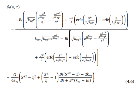
Now, let’s implement this in Mathematica:
In[]:=
θl=-bi-+Erfc-Erfckeq-bi-Exp+Erfc-Erfc--+-1;
keqτ
Exp
-
2
η
4keqτ
η
Exp
-
2
splus
4keqτ
splus
π
2
splus
2
keqτ
η
2
keqτ
keqτ
Exp-1
4keqτ
keqτ
Exp-1
4keqτ
1
splus
-
2
splus
4keqτ
π
2
splus
2
keqτ
1
2
keqτ
G
6keq
2
splus
2
η
splus
η
bi(-1)-2keq
2
splus
bi+splus(keq-bi)
3.2. Temperature distribution in the solid region
3.2. Temperature distribution in the solid region
The dimensionless temperature in the solid region is given by the following expression:

Now, let’s define this in Mathematica:
In[]:=
θs=-(-)+2Sumθi+γExp[-Γτ],{n,1,20};
G
6γ
2
splus
2
η
n+1
(-1)
2
λn
G
2
λn
Sin[λnη]
η
2
λn
3.3. Temperature distribution in the at the solid-liquid interface
3.3. Temperature distribution in the at the solid-liquid interface
The interface position is provided as data points below at various times:
We will fit this data to a smooth polynomial curve. Then, we will use the equation of the resulting curve in our final plot to visualize the melting process. We first input our data into Mathematica in array form:
Let’s now fit this data over a polynomial curve:
A plot for this data can be created as follows:
Note that the interface starts at the initial radius of the PCM, S = 0.05 m. Initially, it decreases rapidly, then slows to a steady linear decline before accelerating towards complete melting at around 80,000 seconds.
The transformation equations that map the dimensionless solutions into their dimensional counterparts are stated below:
We use the Manipulate function of Wolfram Language to visualize the temperature over the melting sphere.
Note: When viewing in cloud, please download this notebook and evaluate it to run the visualization. Here is a static preview of the interactive Manipulate generated above:
This plot shows the temperature over the melting sphere with the slider providing a snapshot of the system at respective times. The light blue color indicates the surrounding liquid medium and the red curve indicates the temperature.
For static comparison, let’s plot the temperature distribution at specific times (0.1 hours, 0.8 hours, 5 hours, 15 hours, and 24 hours). This is shown in Figure 3(a) of the paper [1], and has been reproduced below.
Different snapshots in one figure help us compare the changes in the temperature gradient at specific times during the melting process.
References
References