Wolfram Cloud Document

Introduction

The Hertzsprung–Russell (HR) diagram is one of the most important tools in stellar astrophysics, because it shows that stars do not scatter randomly in temperature-luminosity space. Instead, they cluster into physically meaningful evolutionary regions, including the Main Sequence, Giant Branch, and Supergiant region. In this project, I use supervised machine learning to test whether these classical HR-diagram luminosity classes can be reproduced automatically from real stellar observables. Four features are used as predictors: log effective temperature, log luminosity in solar units, log radius in solar radii, and absolute visual magnitude. The target label is extracted from each star’s spectral class string and simplified into three broad categories: Main Sequence, Giant, and Supergiant. After benchmarking five Wolfram Language classifiers, I select the best-performing model and interpret its behavior using permutation feature importance and HR-diagram decision boundaries.

Data Extraction

All data are retrieved from Wolfram Language’s built-in Star Entity database via EntityClass[“Star”, All] and EntityValue[]. This knowledgebase aggregates data from the Hipparcos catalogue, the Yale Bright Star Catalogue, and the Gliese-Jahreiß Catalogue of Nearby Stars!

Five properties are fetched for every star entity: StellarEffectiveTemperature (K), Luminosity (solar units), StellarRadius (solar radii), AbsoluteMagnitude (dimensionless), and SpectralClass (string). The luminosity class label is extracted from the spectral type string using standard IAU convention: Roman numeral V  MainSequence, III and II  Giant, I (Ia/Ib/Iab)  Supergiant. Temperature, luminosity, and radius are log10-transformed before modelling because each spans several orders of magnitude across the HR diagram.

SeedRandom[51];allStars=EntityList[EntityClass["Star",All]];pool=RandomSample[allStars,Min[30000,Length[allStars]]];spectralRaw=EntityValue[pool,"SpectralClass"];classified=Pick[pool,StringQ/@spectralRaw];Print["Stars with spectral class in pool of ",Length[pool],": ",Length[classified]]starSample=RandomSample[classified,Min[20000,Length[classified]]];Print["Working sample size: ",Length[starSample]]props={"EffectiveTemperature","Luminosity","Radius","AbsoluteMagnitude","SpectralClass"};rawMatrix=EntityValue[starSample,props];cleanMatrix=DeleteMissing[rawMatrix,1,1];Print["First star raw values: ",rawMatrix[[1]]]Print["Number of stars with complete data: ",Length[cleanMatrix]]Print["Working sample size: ",Length[starSample]]

Stars with spectral class in pool of 30000: 27044

Working sample size: 20000

First star raw values: 

6.84×

,Missing[NotAvailable],Missing[NotAvailable],3.07,F2

Number of stars with complete data: 4052

Working sample size: 20000

This extraction step shows that although the Wolfram Star Entity database contains a large pool of stars with spectral classifications, only a smaller subset has all five required physical properties available. From the 30,000-star random pool, 27,044 stars included usable spectral class strings, and 20,000 were selected as the working sample. However, after retrieving temperature, luminosity, radius, absolute magnitude, and spectral class, only 4,052 stars had complete data across all required fields. This is expected because astronomical catalogs often have incomplete measurements, especially for luminosity and radius. Therefore, the final machine learning dataset must be built from the cleaned matrix, not the original 20,000-star sample, to avoid missing-value errors and ensure that every star has both predictor variables and a valid luminosity-class label.

num[x_?NumericQ]:=N[x];num[q_Quantity,unit_]:=Quiet@Check[N[QuantityMagnitude[UnitConvert[q,unit]]],Missing[]];num[x_?NumericQ,unit_]:=N[x];num[_,___]:=Missing[];solarL=3.828*10^26;solarR=6.957*10^8;scale[x_,unit_,factor_]:=Module[{v=num[x,unit]},If[NumericQ[v],v/factor,Missing[]]];lumClass[s_String]:=Which[StringContainsQ[s,"Iab"|"Ia"|"Ib"],"Supergiant",StringContainsQ[s,"III"|"II"],"Giant",StringContainsQ[s,"IV"|"V"],"MainSequence",True,Missing[]];lumClass[_]:=Missing[];makeRow[{t_,l_,r_,mv_,sp_}]:=Module[{temp=num[t,"Kelvins"],lum=scale[l,"Watts",solarL],rad=scale[r,"Meters",solarR],mag=num[mv],cl=lumClass[sp]},If[NumericQ[temp]&&NumericQ[lum]&&NumericQ[rad]&&NumericQ[mag]&&temp>0&&lum>0&&rad>0&&!MissingQ[cl],<|"LogT"->Log10[temp],"LogL"->Log10[lum],"LogR"->Log10[rad],"Mv"->mag,"Class"->cl|>,Nothing]];dataset=makeRow/@rawMatrix;Print["Stars with complete, classifiable data: ",Length[dataset]];classOrder={"MainSequence","Giant","Supergiant"};classCounts=Counts[dataset[[All,"Class"]]];classTable={#,Lookup[classCounts,#,0]}&/@classOrder;Print["Class breakdown:"];Print@Grid[Prepend[classTable,{Style["Class",Bold],Style["Count",Bold]}],Frame->All,Spacings->{2,1}];

Stars with complete, classifiable data: 4021

Class breakdown:

Class	Count
MainSequence	2030
Giant	1904
Supergiant	87

This preprocessing step converts Wolfram Quantity objects into ordinary numerical values, removes stars with missing or nonphysical measurements, applies log transformations to temperature, luminosity, and radius, and extracts the luminosity class from the spectral type string. After filtering, the final dataset contains 4,021 complete and classifiable stars. The class distribution is uneven: Main Sequence = 2,030, Giant = 1,904, and Supergiant = 87. This imbalance is astrophysically expected because supergiants are intrinsically rare, but it also creates an important machine learning issue: the classifier may become better at predicting Main Sequence and Giant stars than Supergiants unless class imbalance is considered during evaluation. Therefore, later model performance should be interpreted using not only overall accuracy, but also class-specific metrics such as precision, recall, or a confusion matrix.

Exploratory Data Analysis

To check whether the cleaned dataset preserves real stellar structure, I first visualized the stars on a Hertzsprung–Russell diagram. The x-axis shows log effective temperature and is reversed so that hotter stars appear on the left, following the traditional astronomical convention. The y-axis shows luminosity in solar units, corrected to log(L/L☉). If the spectral-class parsing worked correctly, Main Sequence stars should form a diagonal band, while Giants and Supergiants should appear above the Main Sequence because they are more luminous.

In[]:=

msStars=Select[dataset,#["Class"]==="MainSequence"&];gStars=Select[dataset,#["Class"]==="Giant"&];sgStars=Select[dataset,#["Class"]==="Supergiant"&];

The dataset is separated by luminosity class before plotting so that each HR-diagram region can be visually checked. This step is important because the machine learning labels come from parsed spectral strings, not manually assigned HR-diagram positions. If the labels are reasonable, the three classes should naturally separate into recognizable astrophysical regions.

cMS=RGBColor[0.18,0.49,0.87];(*blue--MainSequence*)cG=RGBColor[0.93,0.55,0.13];(*orange--Giant*)cSG=RGBColor[0.80,0.14,0.14];(*red--Supergiant*)hrPlot=ListPlot

;densPlot=SmoothHistogram{msStars[[All,"LogL"]],gStars[[All,"LogL"]],sgStars[[All,"LogL"]]},Automatic,"PDF",Filling->Axis,FillingStyle->{Directive[Opacity[0.30],cMS],Directive[Opacity[0.30],cG],Directive[Opacity[0.30],cSG]},

;GraphicsRow[{hrPlot,densPlot},Spacings->30,ImageSize->890]

Out[]=

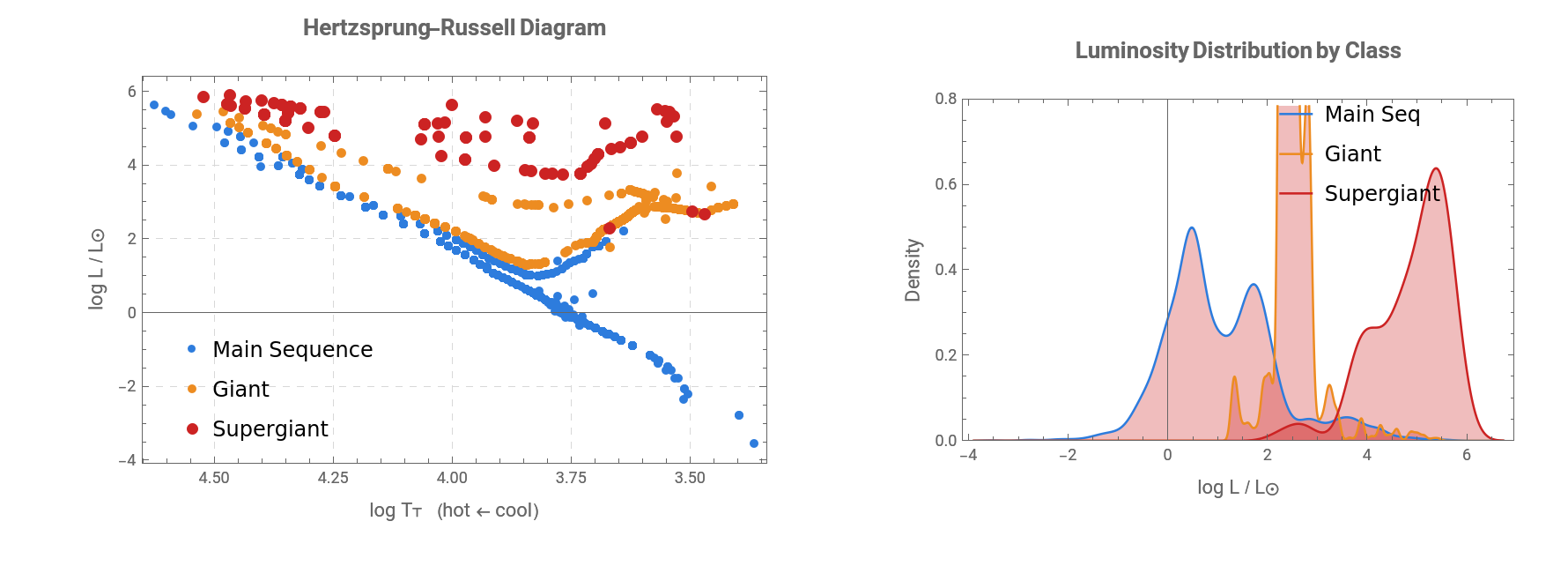
The HR diagram shows the expected structure: Main Sequence stars form a clear diagonal trend from hot, luminous stars to cooler, dimmer stars, while Giants and Supergiants lie above the Main Sequence at higher luminosities. The luminosity-density plot also shows why classification is not perfectly simple. Supergiants are strongly separated at high luminosities, but Main Sequence and Giant stars overlap in some luminosity ranges, meaning luminosity alone cannot fully determine class. This supports the use of multiple predictors — temperature, luminosity, radius, and absolute magnitude — for the machine learning classifier rather than relying only on the HR diagram visually.

Model Training and Benchmarking

To evaluate which machine learning model best reproduces HR-diagram luminosity classification, I benchmarked five Wolfram classifiers using four physical predictors: log temperature, log luminosity, log radius, and absolute magnitude. Because the dataset is class-imbalanced, especially for Supergiants, I used a stratified 80/20 train-test split so that each class remained represented in both training and testing. Macro-averaged precision, recall, and F1 score are reported because they weight Main Sequence, Giant, and Supergiant performance equally rather than allowing the larger classes to dominate the evaluation.

featureKeys={"LogT","LogL","LogR","Mv"};SeedRandom[51];splitClass[cls_]:=Module[{rows,n},rows=RandomSample@Select[dataset,#["Class"]==cls&];n=Max[1,Floor[0.8Length[rows]]];{rows[[;;n]],rows[[n+1;;]]}];{msTrain,msTest}=splitClass["MainSequence"];{gTrain,gTest}=splitClass["Giant"];{sgTrain,sgTest}=splitClass["Supergiant"];train=RandomSample@Join[msTrain,gTrain,sgTrain];test=RandomSample@Join[msTest,gTest,sgTest];Print["Training: ",Length[train]," | Test: ",Length[test]];Print["Test class counts: ",Counts[test[[All,"Class"]]]];

Training: 3216 | Test: 805

Test class counts: Giant381,MainSequence406,Supergiant18

The test set preserves the overall class imbalance while still including Supergiants, the rarest class. This matters because a purely random split could include too few Supergiants in the test set, making the model evaluation less reliable. Stratification makes the benchmark stronger by ensuring that the classifier is tested on all three luminosity classes, not only the more common Main Sequence and Giant stars.

Based on the benchmark table, Random Forest was selected as the final classifier because it achieved the highest accuracy and macro-F1 score among the five tested models. This means it performed best not only overall, but also when the three luminosity classes were weighted more equally. Random Forest is also appropriate for this dataset because HR-diagram classification depends on nonlinear combinations of temperature, luminosity, radius, and absolute magnitude rather than a single clean threshold.

The confusion matrix gives a class-level check of the final Random Forest model. Most predictions fall on the diagonal, meaning the model correctly classifies most Main Sequence stars, Giants, and Supergiants. The remaining errors are physically understandable because Main Sequence stars and Giants can overlap near the boundary between the main sequence and evolved branches, while some luminous Giants can approach the Supergiant region. Since Supergiants are the smallest class, even a few mistakes can noticeably affect recall, so this matrix is necessary to confirm that the high overall accuracy is not hiding weak performance on the rarest class.

Feature Importance

To interpret the final Random Forest model, I used permutation feature importance on the held-out test set. For each feature, I randomly shuffled that feature’s values across the test stars while keeping the other features unchanged, then measured how much the model’s macro-F1 score decreased. A larger drop means the model depended more heavily on that feature for classification. I used macro-F1 instead of raw accuracy because the classes are imbalanced, especially for Supergiants.

The permutation feature importance plot shows that the Random Forest relies most heavily on LogR, followed by LogL, LogT, and finally Mv. This ranking is physically reasonable because luminosity class is strongly connected to stellar evolutionary stage: Main Sequence stars are relatively compact, Giants are expanded, and Supergiants have the largest radii. LogL is also highly important because luminosity separates the upper Giant and Supergiant regions from the lower Main Sequence. LogT adds secondary information by locating stars horizontally on the HR diagram. Mv has the lowest importance because it is partly redundant with LogL; both describe stellar brightness, so once luminosity is already included, absolute magnitude contributes less new information. Because the importance score is based on macro-F1 rather than accuracy, the ranking reflects performance across all three classes, including the rare Supergiants.

Decision Boundaries on the HR Diagram

To visualize the trained Random Forest model, I evaluated it across a dense temperature-luminosity grid and shaded each region by the predicted luminosity class. Because the classifier was trained on four variables, but the HR diagram only shows two dimensions, LogR and Mv are held constant at their training-set means for this visualization. Therefore, the background shading should be interpreted as a two-dimensional slice of the model’s decision behavior, not the full four-dimensional classifier. The real stars are overlaid as colored points to compare the learned boundaries with the physical HR-diagram structure.

The decision-boundary plot shows that the Random Forest learned a physically meaningful version of the HR diagram. The model separates Main Sequence stars from evolved Giants and Supergiants using boundaries that broadly follow the expected stellar evolutionary regions. Main Sequence stars occupy the lower diagonal band, Giants appear above the Main Sequence, and Supergiants dominate the highest-luminosity region. Because this visualization holds LogR and Mv constant, it is only a two-dimensional slice of the full four-feature classifier; the actual model also uses radius and absolute magnitude when making predictions. Overall, the result shows that the classifier is not simply memorizing labels, but learning interpretable patterns from stellar observables.

Conclusion

This notebook demonstrates a full supervised machine learning pipeline for classifying stars into broad HR-diagram luminosity classes using real stellar data from Wolfram Language’s built-in Star Entity database. After extracting and cleaning the data, I converted the physical measurements into machine-learning-ready features: log temperature, log luminosity, log radius, and absolute magnitude. The HR diagram confirmed that the parsed labels were physically meaningful, with Main Sequence stars forming a diagonal band, Giants appearing above the Main Sequence, and Supergiants occupying the highest-luminosity region.

Among the five classifiers tested, Random Forest achieved the strongest overall performance, with the highest accuracy and macro-F1 score. This indicates that the model was able to classify stars accurately while still accounting for the rare Supergiant class. The confusion matrix showed that most errors occurred near physically reasonable boundaries, especially between Main Sequence stars and Giants, where the HR-diagram regions partially overlap.

Permutation feature importance showed that log radius and log luminosity were the most influential predictors, followed by log temperature, while absolute magnitude contributed the least additional information. This ranking makes astrophysical sense because luminosity class is closely tied to stellar size and brightness: Main Sequence stars are relatively compact, Giants are expanded, and Supergiants have the largest radii and luminosities. Finally, the decision-boundary plot showed that the trained Random Forest learned a physically interpretable version of the HR diagram rather than simply memorizing labels. Overall, the project shows that machine learning can reproduce classical stellar classification patterns from real astronomical observables while also revealing which physical features drive the classification most strongly.

You can change the input values and test the classifier yourself. Try making the star hotter, brighter, or larger and see whether the Random Forest changes its prediction from MainSequence to Giant or Supergiant!

CITE THIS NOTEBOOK

Learning the Hertzsprung-Russell diagram: machine learning classification of stellar evolution
by Lim Lee
Wolfram Community, STAFF PICKS, April 27, 2026
https://community.wolfram.com/groups/-/m/t/3706203