Estimation of Kinetic Parameters for Reductive Dechlorination of Chlorinated Solvents
Authors: Housam Binous and Ahmed Bellagi
Estimation of Kinetic Parameters for Reductive Dechlorination of Chlorinated Solvents
Authors: Housam Binous and Ahmed Bellagi
Authors: Housam Binous and Ahmed Bellagi
The pathway of degradation of PCE can be expressed by the following scheme :
PCE → TCE → DCE → VC → ETH
where PCE is tetrachlorethylene and TCE is trichlorethylene, DCE is dichloroethene, VC is vinyl chloride and finally ETH is ethylene.
Derivation of the governing equations is based on the Michaelis - Menten's model.
Kinetic parameters, labelled K1, K2, K3, K4, K5, k1, k2, k3, k4 and k5, are determined using experimental data from Ref. 2.
Here, we present an alternative method, to the one proposed by Balazova et al. (Ref. 1), in order to determine kinetic parameters for reductive dechlorination of chlorinated solvents.
References:
1- Antonia Balazova, Marian Slodicka and Roger Van Keer, Parameter Determination for Reductive Dechlorination of Chlorinated Solvents, Transport in Porous Media, 65, 2006, pp. 411–424.
2- W.M. Wu, J. Nye, R.F. Hickey, M.K. Jain, and J.G. Zeikus. Dechlorination of PCE and TCE to ethylene using an anaerobic microbial consortium. In R.E. Hinchee, A. Leeson, and L. Semprini, editors, Bioremediation of chlorinated solvents, pages 45 - 52. Batelle Pr. Columbus, 1995.
Governing equations are given by the Michaelis-Menten’s model (see Ref. 1) :[t]=-[t]=-[t]=-[t]=-[t]=-where C1, C2, C3, C4 and C5 are the molar concentrations of parent (PCE), intermediate compounds (TCE,DCE and VC) and the final product (ETH), respectively.
′
C1
k1C1[t]
K1+C1[t]
′
C2
k1C1[t]
K1+C1[t]
k2C2[t]
K2+C2[t]
′
C3
k2C2[t]
K2+C2[t]
k3C3[t]
K3+C3[t]
′
C4
k3C3[t]
K3+C3[t]
k4C4[t]
K4+C4[t]
′
C5
k4C4[t]
K4+C4[t]
k5C5[t]
K5+C5[t]
In[]:=
Off[General::"spell1"]
In[]:=
Off[NDSolve::"ndsz"]
In[]:=
Off[InterpolatingFunction::"dmval"]
In[]:=
Off[NDSolve::"ndnum"]
In[]:=
Off[FindMinimum::"lstol"]
Solution of the governing equations when we assume that :
K1=2; K2=5; K3=4; K4=6; K5=10; k1=1; k2=1; k3=2; k4=1 and k5=0.5.
K1=2; K2=5; K3=4; K4=6; K5=10; k1=1; k2=1; k3=2; k4=1 and k5=0.5.
In[]:=
K1=2;K2=5;K3=4;K4=6;K5=10;
In[]:=
k1=1;k2=1;k3=2;k4=1;k5=0.5;
In[]:=
sol=NDSolve[{D[C1[t],{t,1}]-k1C1[t]/(K1+C1[t]),D[C2[t],{t,1}]-k2C2[t]/(K2+C2[t])+k1C1[t]/(K1+C1[t]),D[C3[t],{t,1}]-k3C3[t]/(K3+C3[t])+k2C2[t]/(K2+C2[t]),D[C4[t],{t,1}]-k4C4[t]/(K4+C4[t])+k3C3[t]/(K3+C3[t]),D[C5[t],{t,1}]-k5C5[t]/(K5+C5[t])+k4C4[t]/(K4+C4[t]),C1[0]30,C2[0]0,C3[0]0,C4[0]0,C5[0]0},{C1[t],C2[t],C3[t],C4[t],C5[t]},{t,0,100}]
Out[]=
C1[t]InterpolatingFunction[t],C2[t]InterpolatingFunction[t],C3[t]InterpolatingFunction[t],C4[t]InterpolatingFunction[t],C5[t]InterpolatingFunction[t]


In[]:=
plt1=Plot[Evaluate[C1[t]/.sol],{t,0,100},PlotStyle{Thick,Hue[1/6]},PlotRangeAll];
In[]:=
plt2=Plot[Evaluate[C2[t]/.sol],{t,0,100},PlotStyle{Thick,Hue[2/6]},PlotRangeAll];
In[]:=
plt3=Plot[Evaluate[C3[t]/.sol],{t,0,100},PlotStyle{Thick,Hue[3/6]},PlotRangeAll];
In[]:=
plt4=Plot[Evaluate[C4[t]/.sol],{t,0,100},PlotStyle{Thick,Hue[4/6]},PlotRangeAll];
In[]:=
plt5=Plot[Evaluate[C5[t]/.sol],{t,0,100},PlotStyle{Thick,Hue[5/6]},PlotRangeAll];
In[]:=
Show[plt1,plt2,plt3,plt4,plt5,FrameTrue,GridLinesAutomatic,AspectRatio1,ImageSize400{1,1},FrameLabel{Style["time",14],Style["molar concentration",14]}]
Out[]=
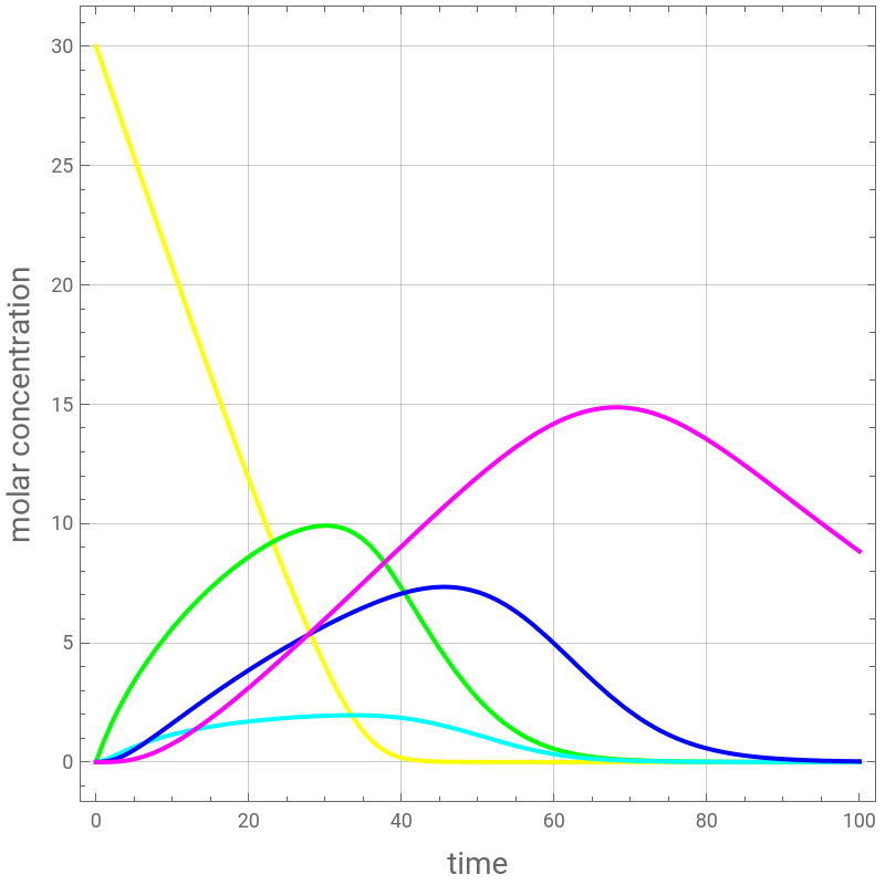
Figure3fromRef.1
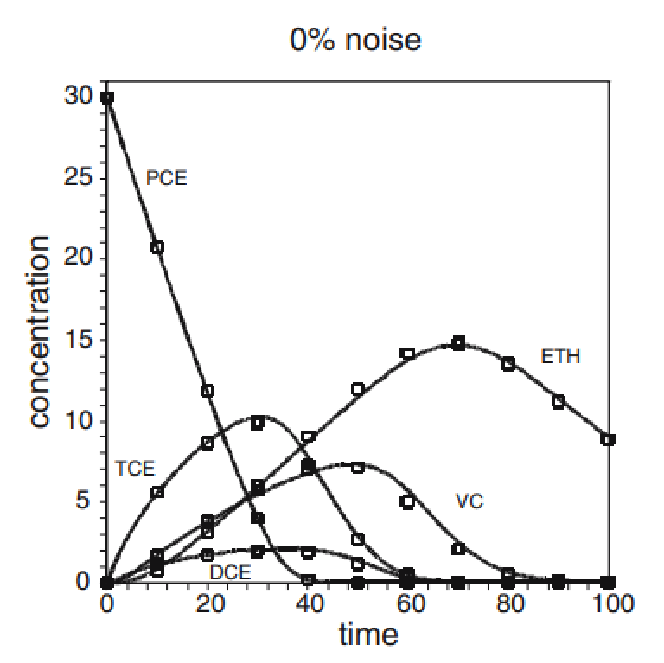
Determination of kinetic parameters K1, K2, K3, K4, K5, k1, k2, k3, k4 and k5 using hypothetical data without noise (0% noise) or hypothetical data with 10% noise.
A set of hypothetical Data is obtained from the above solution {tbl1, tbl2, tbl3, tbl4, tbl5}.
10% noise is added to account for experimental errors {tbl1n, tbl2n, tbl3n, tbl4n, tbl5n}.
A set of hypothetical Data is obtained from the above solution {tbl1, tbl2, tbl3, tbl4, tbl5}.
10% noise is added to account for experimental errors {tbl1n, tbl2n, tbl3n, tbl4n, tbl5n}.
In[]:=
SeedRandom[1234];
In[]:=
tbl1=Table[First[Evaluate[C1[t]/.sol]/.t10i],{i,0,10}]
Out[]=
{30.,20.7384,11.8566,4.01989,0.18434,0.00136106,9.17693×,6.18336×,4.17578×,3.1151×,1.75043×}
-6
10
-8
10
-10
10
-12
10
-14
10
In[]:=
tbl2=Table[First[Evaluate[C2[t]/.sol]/.t10i],{i,0,10}]
Out[]=
{0.,5.61387,8.60192,9.90606,7.3049,2.67012,0.552458,0.0821435,0.0112756,0.00152897,0.000206979}
In[]:=
tbl3=Table[First[Evaluate[C3[t]/.sol]/.t10i],{i,0,10}]
Out[]=
{0.,1.15324,1.70059,1.93751,1.85085,1.13316,0.330644,0.0539293,0.00750222,0.00101905,0.000137981}
In[]:=
tbl4=Table[First[Evaluate[C4[t]/.sol]/.t10i],{i,0,10}]
Out[]=
{0.,1.62572,3.85441,5.71106,7.06066,7.12311,4.96892,2.09962,0.571241,0.122811,0.0244123}
In[]:=
tbl5=Table[First[Evaluate[C5[t]/.sol]/.t10i],{i,0,10}]
Out[]=
{0.,0.765765,3.11254,6.00294,9.03814,11.9517,14.1879,14.8305,13.5329,11.23,8.83131}
In[]:=
tbl1n=Table[First[Evaluate[C1[t]/.sol]/.t10i]+0.1(1-2Random[])First[Evaluate[C1[t]/.sol]/.t10i],{i,0,10}]
Out[]=
{28.913,19.2692,12.0177,3.70036,0.16996,0.00136499,9.07575×,6.69819×,4.58426×,3.23387×,1.70605×}
-6
10
-8
10
-10
10
-12
10
-14
10
In[]:=
tbl2n=Table[First[Evaluate[C2[t]/.sol]/.t10i]+0.1(1-2Random[])First[Evaluate[C2[t]/.sol]/.t10i],{i,0,10}]
Out[]=
{0.,5.69172,8.14709,9.29352,7.33913,2.59364,0.547741,0.0810636,0.011934,0.00144709,0.00020643}
In[]:=
tbl3n=Table[First[Evaluate[C3[t]/.sol]/.t10i]+0.1(1-2Random[])First[Evaluate[C3[t]/.sol]/.t10i],{i,0,10}]
Out[]=
{0.,1.04641,1.8412,1.87588,1.99693,1.23159,0.350711,0.0574512,0.00742685,0.000920808,0.000146656}
In[]:=
tbl4n=Table[First[Evaluate[C4[t]/.sol]/.t10i]+0.1(1-2Random[])First[Evaluate[C4[t]/.sol]/.t10i],{i,0,10}]
Out[]=
{0.,1.48803,3.66072,5.41981,7.62588,7.6726,5.19283,2.26265,0.564724,0.121618,0.0265281}
In[]:=
tbl5n=Table[First[Evaluate[C5[t]/.sol]/.t10i]+0.1(1-2Random[])First[Evaluate[C5[t]/.sol]/.t10i],{i,0,10}]
Determination of kinetic parameters K1, K2, K3, K4, K5, k1, k2, k3, k4 and k5 using data with 10% noise.
We find :
K12.71718,K24.63497,K34.51337,K42.23428,K511.107 and
k11.05042,k20.988463,k32.18352,k40.654384,k50.4965.
If one omits the command SeedRandom[1234], values of parameters will vary slightly depending on the run. Indeed, random data, used to add 10% noise, will be different from run to run.
User may need to change the value of the initial guess of FindMinimum to get correct solution.
We minimize the objective function (sum of the squared deviations). Objective function less than 8.0 .
Computation may take up to several minutes depending on your computer.
Obtained kinetics parameters give concentration profiles that are in agreement with the noisy data used for their determination.