Wei-Prater Mechanism
Authors: Housam Binous and Ahmed Bellagi
Wei-Prater Mechanism
Authors: Housam Binous and Ahmed Bellagi
Authors: Housam Binous and Ahmed Bellagi
References:
[1] G. F. Froment and K. B. Bischoff, Chemical Reactor Analysis and Design, 2rd edition, Wiley, 1990.
[2] James Wei, Charles D. Prater, The Structure and Analysis of Complex Reaction Systems, Editor(s): D.D. Eley, P.W. Selwood, Paul B. Weisz, A.A. Balandin, J.H. De Boer, P.J. Debye, P.H. Emmett, J. Horiuti, W. Jost, G. Natta, E.K. Rideal, H.S. Taylor, Advances in Catalysis, Academic Press, Volume 13, 1962, Pages 203-392.
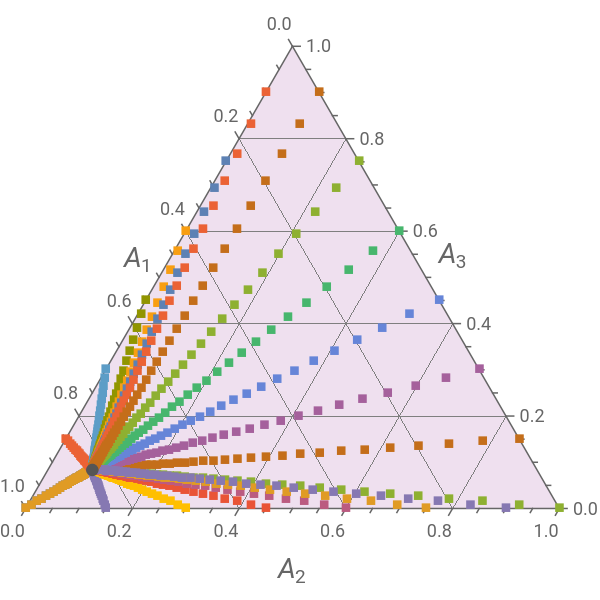
We compute the reaction paths in three-species reaction mixture and plots these paths in an equilateral graph .
This problem was first treated by Wei and Prater in Ref. 2.
Applications of this problem include butene isomerization .
We compute the reaction paths in three-species reaction mixture and plots these paths in an equilateral graph .
This problem was first treated by Wei and Prater in Ref. 2.
Applications of this problem include butene isomerization .
This problem was first treated by Wei and Prater in Ref. 2.
Applications of this problem include butene isomerization .
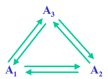
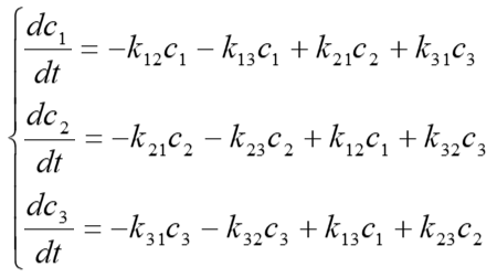
Consider the following complex reaction network, called the Wei–Prater mechanism: .The relevant equations are the following:where is the rate constant of reaction → and =++ is a constant equal to the total concentration of all species for .We display the parametric plots (i.e., versus for different initial conditions) referred to as reaction paths. The system’s steady state is shown with a gray dot; all reaction paths converge to this point. Keep in mind that the rate constants must obey the microscopic reversibility rule or =.
A
1
k
12
⇌
k
21
A
2
k
23
⇌
k
32
A
3
k
31
⇌
k
13
A
1
k
ij
A
i
A
j
C
Total
C
A
1
C
A
2
C
A
3
A
i
i=1,2,3
C
A
1
C
A
2
k
32
k
23
k
12
k
31
k
21
k
13
In[]:=
Sol[a_,b_,c_]:=NDSolve[{D[c1[t],{t,1}]-k12 c1[t]+k21 c2[t]+k31 c3[t]-k13 c1[t],
D[c2[t],{t,1}]k12 c1[t]-k21 c2[t]+k32 c3[t]-k23 c2[t],
D[c3[t],{t,1}]k13 c1[t]-k31 c3[t]-k32 c3[t]+k23 c2[t],c1[0]a,c2[0]b,c3[0]c},{c1[t],c2[t],c3[t]},{t,0,50}]
D[c2[t],{t,1}]k12 c1[t]-k21 c2[t]+k32 c3[t]-k23 c2[t],
D[c3[t],{t,1}]k13 c1[t]-k31 c3[t]-k32 c3[t]+k23 c2[t],c1[0]a,c2[0]b,c3[0]c},{c1[t],c2[t],c3[t]},{t,0,50}]
Numerical values for the rate constants
In[]:=
k12=0.1;k13=0.1;k23=0.1;k21=1;k31=1;
In[]:=
k32=k23k12k31/k21/k13
Out[]=
0.1
Parametric Plot of the species' concentrations
In[]:=
data[a_,b_,c_]:=Table[Evaluate[First[{c2[t],c3[t],c1[t]}/.Sol[a,b,c]]],{t,0,10,0.075}];
Reaction paths in the three-species reaction mixture. Compositions are plotted in an equilateral triangular graph as shown in figure 1.7.2-1 page 44 of G. F. Froment and K. B. Bischoff, Chemical Reactor Analysis and Design, 2rd edition, Wiley, 1990.
In[]:=
TernaryListPlot[Flatten[Table[{data[0.1i,0,0.1(10-i)],data[0.1i,0.1(10-i),0],data[0,0.1i,0.1(10-i)]},{i,10,0,-1.5}],1],PlotMarkersStyle["■",10],ImageSize->300{1,1},GridLines->Automatic,Method->{"Backdrop"LightPurple},FrameLabel->{Style["",14],Style["",14],Style["",14]},PlotRange->All,Epilog->{Darker@Gray,PointSize[0.0225],Point[Last@data[0.1,0,0.1(10-1)]]}]
A
2
A
3
A
1
Out[]=