Statistical patterns on MIT OpenCourseWare’s YouTube channel
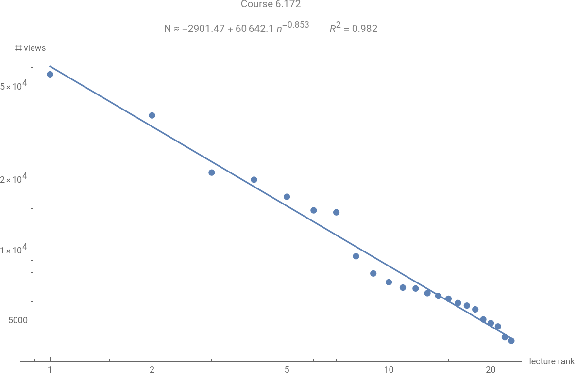
The current essay analyzes the number likes, dislikes, and views at MIT OpenCourseWare’s YouTube channel, where some of MIT’s courses are published. The essay looks at 95 courses. An interesting pattern is that some lectures typically have significantly more likes and views than the other lectures in the same course. In the course 22.01: Introduction to Nuclear Engineering and Ionizing Radiation, for example, the most popular lecture has 185 times more views than the median! And the number of views of the -th most popular lecture in any of the surveyed courses is very accurately ) described by a power law for some constants , , , which are unique for each course, and . It turns out that the average value of is roughly 1, which is reminiscent of Zipf’s law. This suggests that most of the views that MIT OCW’s YouTube channel gets come from “laymen” who randomly click the videos rather than students who methodically watch the videos one by one. This conclusion is confirmed by the fact that courses with loud names, such as Introduction to Nuclear Engineering and Ionizing radiation, have a higher variability of views than courses with modest names like Introduction to Solid State Chemistry. While loud names attract many laymen, courses with modest names are mostly viewed by students who systematically watch the lectures. The current essay also compares different majors. Materials science and physics courses were found to have a very high ratio of likes to dislikes, contrary to architecture and urban science & planning. The majors with the highest ratio of likes to views are Nuclear Science and Cognitive Science, and the most popular majors are math and computer science. The majors with the highest unevenness, or variability, in the number of views are Nuclear Science and Biological Engineering, which can be explained by the fact that their content has been “hyped up” by science fiction. As a final note, the reasons for choosing MIT OpenCourseWare as the subject of study (as opposed to, for example, EdX) were: (1) OCW is the largest of its kind, (2) MIT uses a particularly simple course naming system, (3) MIT OpenCourseWare’s YouTube channel is more popular than its competitors’.
n
(≈0.97
2
R
N≈+k
-γ
n
k
γ
||<<k
γ
Out[]=
Average ratio of likes to dislikes for different majors |
















Out[]=
Extracting the data
Extracting the data
Before beginning to analyze the data, we need to first gather it. This step is quite trivial, so reading this section is not that important. Now, getting to the technical part, getVideos returns the list of links to all videos in a given playlist, and videoData returns the number of likes, dislikes, and views for a given video. Together, they can be used to determine the number of likes and and dislikes for all videos in a given playlist. And since lecture courses come in the form of playlists, we can use the functions to find the number of likes, disliked, and views (later called the data) for a given course. What then remains is to make a list of courses and run the program. And lastly, it must be noted that the two functions below only work in Kazakhstan because they assume that the language of the YouTube page is Kazakh. If you run this from somewhere else - Europe, the US, Asia, etc - you would need to figure out what keywords to use when parsing the HTML text. This can be done within 30 minutes by opening some random video and looking through the HTML code of the YouTube player. If the number of views is 47329, then in the HTML you should look for the number 47329. The structure of the page is the same for all videos, so it’s possible to deduce a general rule for finding the data on the video.
In[]:=
ClearAll[getVideos];getVideos[playlist_] := Block[ text = URLRead[playlist]["Body"], shift, truncatedText, marker = "\"title\":{\"runs\":[{\"text\":", markerLen, markerChars, antimarker = "\"YouTube TV\"", antimarkerLen, antimarkerChars, record = True, markerPositions, i, iHelper, j , markerLen = StringLength[marker]; markerChars = Characters[marker]; antimarkerLen = StringLength[antimarker]; antimarkerChars = Characters[antimarker]; shift = StringPosition[text, marker][[1, 1]] - 1; truncatedText = StringJoin@StringPart[text, shift + 1;;]; markerPositions = StringPosition[truncatedText, marker][[All, 2]]; Table[ If[StringPart[truncatedText, pos+1;;pos + antimarkerLen] antimarkerChars, record = False]; If[record, iHelper = False; For[i = pos, True, i++, If[StringPart[truncatedText, i;;i + 2] {"u", "r", "l"}, If[iHelper, Break[], iHelper = True]] ]; For[j = i, True, j++, If[StringPart[truncatedText, j] ",", Break[]] ]; "https://www.youtube.com" <> StringJoin[StringPart[truncatedText, i+6;;j-2]], Nothing ], {pos, markerPositions} ]]
In[]:=
ClearAll[getVideoData];getVideoData[video_] := Block[ text = URLRead[video]["Body"], likesStart, i, dislikesStart, j, viewsStart, k , likesStart = StringPosition[text, "Басқа "][[1, 2]] + 1; For[i = likesStart, StringPart[text, i] ≠ " ", i++, Null]; dislikesStart = StringPosition[text, "басқа "][[1, 2]] + 1; For[j = dislikesStart, StringPart[text, j] ≠ " ", j++, Null]; viewsStart = StringPosition[text, "\"viewCount\":\""][[1, 2]] + 1; For[k = viewsStart, StringPart[text, k] ≠ "\"", k++, Null]; k--; ToExpression@StringJoin@StringPart[text, viewsStart;;k], ToExpression@StringJoin@StringPart[text, likesStart;;i], ToExpression@StringJoin@StringPart[text, dislikesStart;;j] ]
List of courses
List of courses
Extract data from YouTube channel
Extract data from YouTube channel
Here is the code that extracts the data from the YouTube channel:
In[]:=
ytData={#[[1]],getVideoData/@getVideos[#[[2]]]}&/@courseList;
In[]:=
ytData
Out[]=
And since it takes forever to run, I’ve recorded the output it produces and copied it into the notebook like that, so that the code would not have to be executed every time:
It must be noted that the data above was gathered in January 2021, so by the time you read the essay, the actual numbers might change. ytData is a list of the form {..., {name, {lec1, lec2, ... }}, ...}, where name is the name of a course and lec1 represents the first lecture in the course. lec1 is of the form {views, likes, dislikes}.
The student-layman model and Zipf’s law
The student-layman model and Zipf’s law
Introducing the model
Introducing the model
The first thing that we notice when looking at the number of views for the lectures in a given course is that the numbers are highly uneven. Here, for example, is the data for the course 6.172:
Interesting features
Interesting features
Interpretation
Interpretation
Comparing courses
Comparing courses
Max to median views
Max to median views
Total views
Total views
Let’s now assess courses’ popularity by comparing their total number of views:
The most popular course is 6.006: Introduction to Algorithms, and the next most popular one is 18.06: Linear Algebra. These courses are relevant in fields like machine learning and IT, as well as a ton of other industries - probably that’s why they are so popular. Notice that the first seven positions are taken by math and computer science as the most “industrious” fields. The first non-math and non-CS popular courses are 8.04: Quantum mechanics I and 14.01SC: Principles of Microeconomics. The three least popular courses are 4.696: A Global History of Architecture, 3.091: Introduction to Solid State Chemistry and 11.601: Introduction to Environmental Policy and Planning. These are courses with very specific target audience and a comparatively limited practical application (apart from 3.091, which strangely has so few views). It is interesting that 6.S897, a computer science course, is the fifth least popular course, as CS is the most popular major. The explanation is probably that the course is very specific: its name is Machine Learning for Health Care, which is only going to attract a few narrow specialists. All in all, it can be seen that majors relevant in industry, such as computer science and math, are the most popular, while courses with a narrow target audience and comparatively limited practical applications get the least number of views.
Likes to dislikes
Likes to dislikes
Having assessed the courses’ popularity, it would now be interesting to evaluate how enjoyable they are by comparing the total number of likes to the total number of dislikes they have. The idea is that the more exciting is the course, the higher is the ratio of likes to dislikes. There are of course some issues with this metric - for example, since there are far more laymen than students, the data we get will reflect the preferences of laymen - it’s still a fairly reasonable way to measure how exciting the course’s content is. So, here is the code:
Likes to views
Likes to views
Lastly, let us assess the “level of devotion” of the viewers - that is, what proportion of the viewers bother to press the “like” button. The idea is that the more engaged the viewers are, the more likely they are to press “like”.
The leading course is 3.091: Introduction to Solid State Chemistry, with over two percent of viewers pressing the “like” button. It is closely followed by 9.40: Introduction to Neural Computation and 15.S08: Shaping the Financial World. The courses with the least engaged viewers, with only 0.1% bothering to press “like”, is 6.451: Principles of Digital Communication II. The next least engaging course is 6.033: Computer System Engineering, also a CS course. Although computer science is the most popular course, its viewers seem to be the most disengaged. Also, notice that the course 3.091 has appeared several times as the number one course in several charts; it seems to be a really exciting course.
Comparing majors
Comparing majors
Introduction
Introduction
For the course 15.S08, for example, it returns 15:
We can use this function to find the list courseMajors of all majors in the dataset, as well as the Association (similar to a dictionary) coursesByMajor, which for each major gives the courses that belong to it. The format of coursesByMajor is <..., |majorCode -> {course1Id, course2Id, ...}|, ...>, where {course1Id, course2Id, ...} is the list of all courses in the major with code majorCode (the list may have just one element):
Likes to dislikes
Likes to dislikes
Now that we have arranged the courses by majors, we can actually start looking for patterns. First, let’s compare the average ratio of likes to dislikes for a given major, which would (roughly) tell us the degree to which YouTube viewers like a particular major. One way to define this quantity is to compute the mean ratio of likes to dislikes among all the courses of a particular major. For instance, if the (fictional) major Sunset Observation has two courses in it, and their respective ratios of likes to dislikes are 80.3 and 92.4, then the average ratio of likes to dislikes of the major Sunset Observation is 86.35. This definition is good in that all courses have equal weight, independently of their popularity. So, here is the function that computes the ratio of likes to dislikes for a given major:
The list is of the form {major1Id, major2Id, ...}. It gives the id’s of the majors, which we can then convert to names using the list courseMajors. Here is the table showing the names of majors and their average ratio of likes to dislikes:
And here is a more colorful chart, with major codes replaced by names:
Materials science is again on top, and architecture is again last. Physics comes the second, and then goes Cognitive studies and Biology. Engineering (all five varieties) are at the bottom, together with Nuclear science and Planning.
Likes to views
Likes to views
Now, let’s compare majors by likes to views. As in the previous subsection, let us define
As previously, Architecture is at the very bottom. However, now the chart is topped by Nuclear science, which is actually one of the worst courses by the ratio of likes to dislikes.
Maximum to median views
Maximum to median views
Repeating the procedure for the ratio of the maximum number of views to the median, we obtain the following result:
As many times before, Architecture is at the very bottom; this indicates that the maximum number of views is fairly close to the median, which means that there are relatively few laymen watching the course. Nuclear science is way above the rest of the courses, with the average ratio of max to median being 185. This implies that the major attracts many laymen, which makes sense if you consider that the course’s name is rather loud and its content has been widely advertized by sci-fi.