One of the brightest characteristics of the Wolfram Language (WL) is that it works easily across many different scientific fields (thanks to numerous built-in functions and data) and that due to the coherence of WL design, combining such different sciences via computation comes as natural as speaking to a human. Here WL will enable us to move quickly from computational geometry to machine learning to statistics on a quest of exploring an interesting subject. This seemingly simple question is not easy to answer without right framework and tools:
What is statistical distributions of areas of cells in Voronoi tessellation?
From a brief web search it appears to follow closely GammaDistribution. But in the absence of analytical proof, how can one quickly deduce this fact or verify it is good model? We will do exactly that below. For reference see also a relevant paper by TANEMURA and a real-interest question by actual user which prompted this exploration.
To start let’s build a “large” VoronoiMesh on 5000 uniformly distributed points within a unit Disk:
pts=RandomPoint[Disk[],5000];
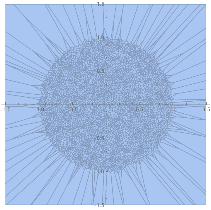
We see the statistics we can gather from this will be obviously offset by the presence of “border” cells of much larger area than regular inner cells have:
mesh=VoronoiMesh[pts,AxesTrue]
Out[]=
Let’s exclude large cells by selecting only those within original region of random points distribution - unit Disk:
In[]:=
vor=MeshPrimitives[mesh,2];vor//Length
Out[]=
5000
In[]:=
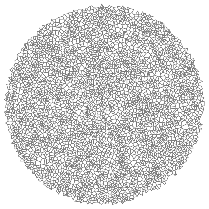
vorInner=Select[vor,RegionWithin[Disk[],#]&];vorInner//Length
Out[]=
4782
We got fewer elements of course and they all are nice regular cells without any large outliers:
In[]:=
Graphics[{FaceForm[None],EdgeForm[Gray],vorInner}]
Out[]=
Let’s take a look at the statistics of areas’ distribution:
In[]:=
areas=Area/@vorInner;hist=Histogram[areas,Automatic,"PDF",PlotTheme"Detailed"]
Out[]=
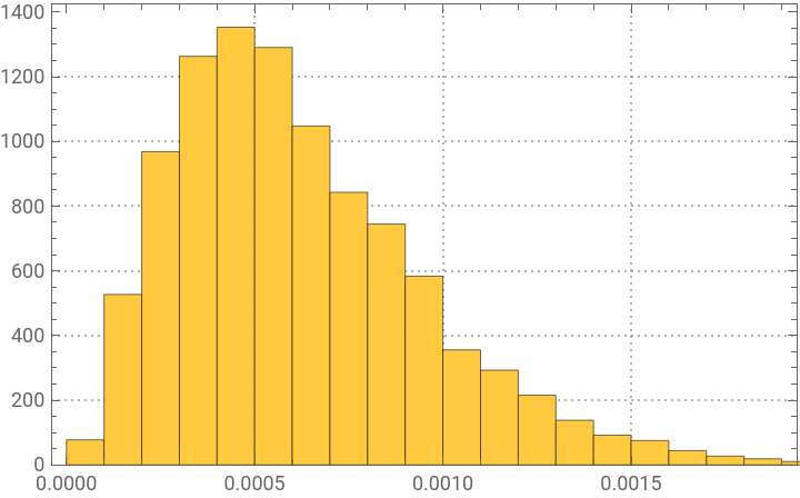
We can see that there is a minimum of distribution at zero area, which is intuitively correct. Close to zero-area cells of course are not present much with the finite number of points per region (or finite density). So there is some prevalent finite mean area there. We can find a very close simple analytic distribution using WL machine learning tools, which turns out to be GammaDistribution as discussed in some publications:
In[]:=
dis=FindDistribution[areas]
Out[]=
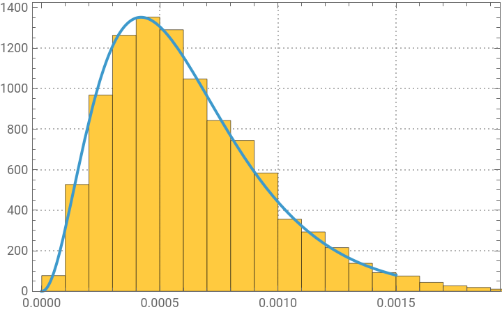
GammaDistribution[3.19022,0.000191989]
FindDistribution acted automatically without any additional options from our side. GammaDistribution matches very nicely the empirical histogram:
In[]:=
Show[hist,Plot[PDF[dis,x],{x,0,.0015}]]
Out[]=
And now it is easy to find thing like:
In[]:=
{Mean[dis],Variance[dis],Kurtosis[dis]}
Out[]=
{0.000612488,1.17591×,4.88075}
-7
10
In[]:=
Probability[x>.0005,xdis]
Out[]=
0.563507
CITE THIS NOTEBOOK
CITE THIS NOTEBOOK
Statistical distributions of areas of Voronoi cells
by Vitaliy Kaurov
Wolfram Community, STAFF PICKS, 2019
https://community.wolfram.com/groups/-/m/t/1620190
by Vitaliy Kaurov
Wolfram Community, STAFF PICKS, 2019
https://community.wolfram.com/groups/-/m/t/1620190