Variational Quantum Eigensolver
Variational Quantum Eigensolver
The Variational Quantum Eigensolver (VQE) is a quantum algorithm designed to find the ground state energy of a Hamiltonian, which is central to many quantum chemistry and physics problems.
Load Quantum Framework
Load Quantum Framework
Using Wolfram Quantum Framework
In[]:=
PacletInstall["https://wolfr.am/DevWQCF",ForceVersionInstall->True]
Out[]=
PacletObject
In[]:=
<<Wolfram`QuantumFramework`
Load QuantumOptimization paclet
In[]:=
<<Wolfram`QuantumFramework`QuantumOptimization`
Functionalities
In[]:=
?Wolfram`QuantumFramework`QuantumOptimization`*
Out[]=
Theory
Theory
Definition
Definition
The variational principle provides an upper bound to the lowest possible expectation value of an observable with respect to a trial wavefunction The ground state energy associated with a Hamiltonian is bounded as follows:
|ψ〉.
E
o
H
E 0 〈ψ| H ψ ψ |
In this equation:
◼
E
0
◼
H
◼
|ψ〉
◼
ψ
ψ
Objective
Objective
The goal of the VQE is to find a parameterized form of the wavefunction such that the expectation value of the Hamiltonian is minimized.
|ψ〉
In other words, we need to find such that
|ψ〉≡ψ
θ
opt
->
H
E
0
This expectation value forms an upper bound to the ground state energy, and ideally, it should match the true ground state energy to the desired precision.
Mathematically, the objective is to approximate the eigenvector of the Hermitian operator H that corresponds to the lowest eigenvalue, .
|ψ〉
E
0
Implementation
Implementation
To solve this optimization problem on a quantum computer, we need to define a parameterized ansatz (a trial wavefunction) that can be implemented as a series of quantum gates. This is crucial because quantum computers can only perform unitary operations or measurements.
◼
Ansatz Wavefunction
◼
The wavefunction is expressed as the application of a generic unitary operation to an initial state in every qubit.
|ψ〉
U(θ)
|0〉
◼
After defining the ansatz, the optimization problem for the VQE becomes:
E VQE min θ † U H |
where U(θ) is an ansatz conformed by unitary gates with .
θ∈(-π,π]
This expression is often referred to as the cost function of the VQE. The objective is to minimize this cost function with respect to the parameters θ.
Once the parameters θ are optimized, we obtain the lowest possible energy (the ground state energy) for the system represented by the Hamiltonian H.
This is a variational approach because it optimizes an upper bound of the true ground state energy, which is the core idea behind the algorithm.
Toy H2 Molecule
Toy Molecule
H
2
The current problem is finding the ground state of the molecule;,the Hamiltonian can be reduced and modeled using two qubits as:
H
2
In[]:=
H2=QuantumOperator[α("ZI"+"IZ")+β*"XX"]
Out[]=
QuantumOperator
Implement the algorithm as we learned last class:
◼
First: Parametrized quantum circuits, state and ansatz preparation.
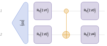
In this case we will use a typical hardware-efficient ansatz: Two layers of Rotations and a CNOT to ensure the entanglement.
In[]:=
HEAnsatz=QuantumCircuitOperator[{"00","RY"[2θ1]->1,"RY"[2θ2]->2,"CNOT"->{1,2},"RY"[2θ3]->1,"RY"[2θ4]->2}];HEAnsatz["Diagram"]
Out[]=
◼
Second: Cost function
〈H(θ)〉
We need a cost function, so let’s obtain the QuantumState from the QuantumCircuit and define the bra and ket.
In[]:=
|ϕ〉=HEAnsatz[];〈ϕ|=;
†
|ϕ〉
Finally lets compute the energy of our system and define a function that will work as the cost function. In this step we should help the optimizer by Simplifying and replacing fixed values.
In[]:=
energy=〈ϕ|@H2@|ϕ〉;
In[]:=
values={α->0.4,β->0.2};costH2[θ1_,θ2_,θ3_,θ4_]=FullSimplify["Scalar"//energy,{θ1,θ2,θ3,θ4}∈Reals]/.values
Out[]=
Sin[2θ1](0.2Cos[2θ3]Cos[2θ4]-0.4Sin[2θ2]Sin[2θ3])+Cos[2θ1](0.4Cos[2θ3]+Cos[2θ4](0.4Cos[2θ2]+0.2Sin[2θ2]Sin[2θ3]))+(-0.4Sin[2θ2]+0.2Cos[2θ2]Sin[2θ3])Sin[2θ4]
As I mentioned, the cost function we are working with is not trivial, but the advantage is that we can compute it symbolically, which significantly helps in the optimization process.
◼
Third: Optimization
To find the optimal parameters for our quantum circuit, we can use the NMinimize function in Mathematica.
In[]:=
resultH2=NMinimize[costH2[θ1,θ2,θ3,θ4],{θ1,θ2,θ3,θ4}]
Out[]=
{-0.824621,{θ10.717444,θ2-0.909051,θ3-0.855457,θ42.37329}}
This function allows us to minimize the cost function by adjusting the parameters, and after performing this minimization, we obtain the optimized parameters and the minimum value of the cost function, which in this case is approximately -0.824.
In[]:=
paramH2=Last[resultH2]//Association
Out[]=
θ10.717444,θ2-0.909051,θ3-0.855457,θ42.37329
Now that we have the optimal value, it is insightful to inspect the behavior of the cost function around these points. Since we have four variables (the parameters in the ansatz), we need to fix two of the values in order to visualize the function.
We can do this by using a ContourPlot, which will allow us to observe the shape of the cost function in two dimensions.
In[]:=
ContourPlot[costH2[θ1,θ2,paramH2[θ3],paramH2[θ4]],{θ1,-π/2,π/2},{θ2,-π/2,π/2},FrameLabel->Automatic]
Out[]=
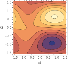
ContourPlot is useful here because it highlights where the cost function attains higher and lower values. In this plot, the lighter sections correspond to higher values, and the blue sections represent the lowest values of the cost function.
In[]:=
ContourPlot[costH2[θ1,paramH2[θ2],θ3,paramH2[θ4]],{θ1,-π/2,π/2},{θ3,-π/2,π/2},FrameLabel->Automatic]
Out[]=
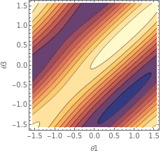
If the optimization algorithm has started with a point near the blue section (where the minimum lies), we can expect it to converge towards this blue region, as this represents the optimal set of parameters. The algorithm searches for regions where the cost is minimized, and this plot helps visualize the “shape” of the function.
When the cost function is relatively simple and can be expressed symbolically, the ContourPlot can exhibit repetitive patterns. This repetition often results from the periodic nature of trigonometric functions (e.g., sinand cos) that may appear in the cost function due to the rotation gates used in the ansatz.
Example from https://arxiv.org/pdf/1909.05074v1
Quantum Chemistry
Quantum Chemistry
The Variational Quantum Eigensolver (VQE) is a valuable tool in quantum chemistry for finding the minimal energy of a molecule. The task is essentially an optimization problem, where the goal is to minimize the total energy of the molecule with respect to the positions of the atomic nuclei.
In the case of VQE, we use parameterized quantum circuits to approximate the ground state energy of the system. This results in the determination of the minimal energy of the system, which corresponds to the lowest energy configuration of the molecule in its ground state.
This minimal energy result can be incredibly useful in determining the geometry of the molecule as well, as the lowest energy corresponds to the optimized configuration of the atomic nuclei. Therefore, although the main goal is to minimize the energy, this process can also provide insights into the stable arrangement of atoms in the molecule.
Trihydrogen cation
Trihydrogen cation
First we will use some python code from PennyLane to obtain the Hamiltonian corresponding to the H3 cation.
We just need to indicate the molecules “H” and the coordinates:
In[]:=
import pennylane as qml
from pennylane import numpy as np
symbols = ["H", "H", "H"]
coordinates = np.array([0.028, 0.054, 0.0, 0.986, 1.610, 0.0, 1.855, 0.002, 0.0])
# Building the molecular hamiltonian for the trihydrogen cation
hamiltonian, qubits = qml.qchem.molecular_hamiltonian(symbols, coordinates, charge=1)
qml.matrix(hamiltonian)
In case Python is not available, you can import it from this location:
Finally we obtain a NumericArray which we will turn into a QuantumOperator:
If we have no prior knowledge of the structure of the circuit, a reasonable starting point could be a layered circuit consisting of rotations around the Y-axis and CNOT gates.
To encode the occupation numbers of the molecular spin-orbitals, we would need six qubits.
If you’d like to learn how to construct layered circuits using ParametrizedLayer and EntanglementLayer please refer to the Quantum Optimization documentation.
In this case, you can expect a very complex symbolic cost function. To handle this, we could choose to implement a numerical function instead.
We begin by using Module to define the quantum state with parameters replaced by real numbers. Next, we define the ket and bra, and then compute the scalar resulting from the expectation value of the Hamiltonian H.
After defining the cost function, we can apply a classical optimizer starting from an initial guess to find the minimum energy value.
If we are interested in obtaining the geometry of the system, we would need to introduce a parameterized Hamiltonian for optimization as well, to optimize both the energy and the geometry.