ORIGINAL ARTICLE: S Silliman and M Bhattacharya (2023), (Avoided) crossings in the spectra of matrices with globally degenerate eigenvalues, Eur. J. Phys. 44 065403. DOI: https://doi.org/10.1088/1361-6404/acfbc4
Article Abstract: (Avoided) crossings are ubiquitous in physics and are connected to many physical phenomena such as hidden symmetries, the Berry phase, entanglement, Landau–Zener processes, the onset of chaos, etc. A pedagogical approach to cataloging (avoided) crossings has been proposed in the past, using matrices whose eigenvalues avoid or cross as a function of some parameter. The approach relies on the mathematical tool of the discriminant, which can be calculated from the characteristic polynomial of the matrix, and whose roots as a function of the parameter being varied yield the locations as well as degeneracies of the (avoided) crossings. In this article we consider matrices whose symmetries force two or more eigenvalues to be degenerate across the entire range of variation of the parameter of interest, thus leading to an identically vanishing discriminant. To show how this case can be handled systematically, we introduce a perturbation to the matrix and calculate the roots of the discriminant in the limit as the perturbation vanishes. We show that this approach correctly generates a nonzero ‘reduced’ discriminant that yields the locations and degeneracies of the (avoided) crossings. We illustrate our technique using the matrix Hamiltonian for benzene in Hückel theory, which has recently been discussed in the context of (avoided) crossings in its spectrum.
Introduction
Introduction
Crossings and avoided crossings between the eigenvalues of a matrix, as a system parameter is varied, are ubiquitous in physics and mathematics. They are relevant to the studies of hidden symmetries, the Berry phase, entanglement, Landau-Zener processes, chaos, the Born-Oppenheimer approximation, etc.. This notebook is an introduction to a systematic and powerful method, superior to mere inspection of the eigenvalue spectrum, of locating (avoided) crossings using the built-in function Discriminant in Mathematica.
Toolbox: Relevant properties of the Discriminant
Toolbox: Relevant properties of the Discriminant
Here we list, without proof, the properties of the discriminant we will use [1]. For a matrix H(P) depending on the parameter P, the discriminant D[H(P)] can always be found analytically from the characteristic polynomial of H(P), and:1. The real roots of D[H(P)] correspond to crossings.2. The real parts of the complex roots of D[H(P)] correspond to avoided crossings.3. Each (avoided) crossing gives rise to a factor in D[H(P)] quadratic in P.4. A crossing is defined as the intersection of two eigenvalues. Therefore the simultaneous intersection of m eigenvalues leads to = m(m-1)/2 crossings. 5. If H(P) is Hermitian, D[H(P)] ≥ 0. Thus Log [D[H(P)]+1]≥ 0 and vanishes at every crossing.
m |
2 |
Simple example: A 2 x 2 matrix
Simple example: A 2 x 2 matrix
Consider the matrix [1]
In[]:=
H0={{E1,V},{V,E1}};MatrixForm[H0]
Out[]//MatrixForm=
E1 | V |
V | E1 |
Find its characteristic polynomial
In[]:=
P0=CharacteristicPolynomial[H0,λ]
Out[]=
2
E1
2
V
2
λ
Find its discriminant
In[]:=
D0=Discriminant[P0,λ]
Out[]=
4
2
V
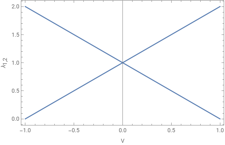
Using Tools 1, 2, 3 and 4 above we can conclude that there is only a single crossing at V = 0. There are no avoided crossings. We can check this for specific values of the parameters by plotting the spectrum:
In[]:=
Plot[Eigenvalues[H0]/.{E1->1},{V,-1,1},Frame->True,FrameLabel->{"V","SubscriptBox[\(λ\), \(1, 2\)]"}]
Out[]=
Higher dimensional matrices
Higher dimensional matrices
Now consider the 4 x 4 matrix [1]
In[]:=
H1={{A-2(a+b)B,0,0,0},{0,-A+2(a-b)B,2A,0},{0,2A,-A-2(a-b)B,0},{0,0,0,A+2(a+b)B}};MatrixForm[H1]
1
4
Out[]//MatrixForm=
1 4 | 0 | 0 | 0 |
0 | 1 4 | A 2 | 0 |
0 | A 2 | 1 4 | 0 |
0 | 0 | 0 | 1 4 |
This matrix describes the ground spin state of the Hydrogen atom in a magnetic field. A, B, a and b are the hyperfine splitting, magnetic field, and electron and proton magnetic constants, respectively.
b = 0
b = 0
For b = 0, we find the matrix takes the form
In[]:=
H1b=H1/.{b->0};MatrixForm[H1b]
Out[]//MatrixForm=
1 4 | 0 | 0 | 0 |
0 | 1 4 | A 2 | 0 |
0 | A 2 | 1 4 | 0 |
0 | 0 | 0 | 1 4 |
The corresponding discriminant is
In[]:=
P1b=CharacteristicPolynomial[H1b,λ];D1b=Simplify[Discriminant[P1b,λ]]
Out[]=
1
16
6
a
4
A
6
B
2
A
2
a
2
B
If we consider the magnetic field B as the parameter being varied, the compact polynomial D1b tells us that:1. There is a 6-fold root at B=0. According to Tool 3, this corresponds to 3 eigenvalues crossing at B=0, since contributes a factor of to the discriminant.2. There are two complex roots at B = ± i. Since the real part of this conjugate pair is zero, according to Tools 2 and 3, there is a single avoided crossing at B=0. 3. The hyperfine splitting A is physically responsible for the avoided crossing, since if A=0, the avoided crossing will become a crossing. If you like (not necessary for the method!) we can use specific values of the parameters to plot the spectrum:
=3andeachcrossing
3 |
2 |
2
B
A
a
In[]:=
Plot[Eigenvalues[H1b]/.{A->0.5,a->0.8},{B,-1,1},Frame->True,FrameLabel->{"B","SubscriptBox[\(λ\), \(1, 2, 3, 4\)]"}]
Out[]=
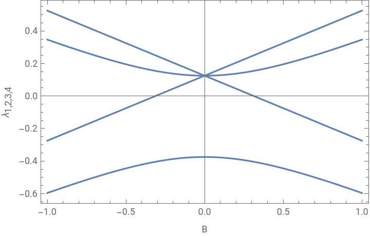
Please note the parameter values are chosen for convenience of plotting and do not correspond to those found in nature.
b ≠ 0
b ≠ 0
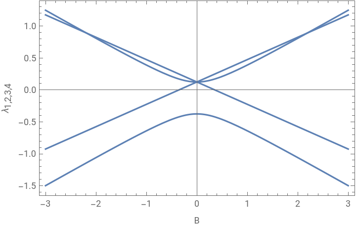
In this case we will leave the explicit form of the discriminant to the references posted below [1]; instead we will show how the discriminant is a useful tool for visualization of crossings. For b ≠ 0, additional crossings show up in the spectrum for B ≠0. They cannot be located too easily in the spectrum, but a plot of the discriminant, using Tool 5, pinpoints them more clearly (this method gains in power when there are several crossings close by):
In[]:=
Plot[Eigenvalues[H1]/.{A->0.5,a->0.8,b->-0.1},{B,-3,3},Frame->True,FrameLabel->{"B","SubscriptBox[\(λ\), \(1, 2, 3, 4\)]"}]
Out[]=
In[]:=
P1=CharacteristicPolynomial[H1,λ];D1=Discriminant[P1,λ];
In[]:=
PlotLog[Evaluate[D1/.{A->0.5,a->0.8,b->-0.1}]+1],{B,-3,3},Frame->True,FrameLabel->{"B","Log[N D1+1]"},PlotRange->All
15
10
Out[]=
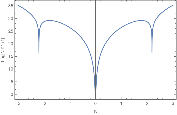
Note that on the y-axis label a scale factor can be tweaked to improve contrast.
N=
15
10
What if the discriminant vanishes identically?
What if the discriminant vanishes identically?
What if the discriminant vanishes identically? This happens when two or more eigenvalues happen to be degenerate throughout the entire range of variation of the parameter of interest. Consider, as an example, the matrix [2]
This matrix describes the molecule benzene. a is the tunable parameter. Let’s plot the spectrum:
We see only 4 eigenvalues, whereas there should be 6 (equal to the dimension of the matrix H2). Clearly there are (avoided) crossings in the spectrum, but if we calculate the discriminant, we find that it vanishes identically for any value of a
A systematic way to fix this problem is to add a perturbation to the matrix H2 that removes the global degeneracy. Let’s try the simplest perturbation we can think of:
Adding Hp to H2, we plot the spectrum again, for, say, ϵ = 0.5.
Now the all global degeneracies are removed, and we see 6 eigenvalues. Let’s find the corresponding discriminant (for any ϵ).
Now let us find the roots of Dn
Mathematica gives some roots explicitly, and some as root objects. Let us take the limit of vanishing perturbation ϵ → 0:
It can be confirmed, using Tools 1-4, that these roots correctly signify, in the unperturbed spectrum shown above
1. One crossing at a = -1.
2. Four crossings at a = 0.
3. Four avoided crossings at a = 1/2.
A ‘reduced’ discriminant can be constructed, using these roots, to describe the system [2].
1. One crossing at a = -1.
2. Four crossings at a = 0.
3. Four avoided crossings at a = 1/2.
A ‘reduced’ discriminant can be constructed, using these roots, to describe the system [2].
References
References
[1] M. Bhattacharya, Am. J. Phys. 75, 942 (2007).
[2] S. Silliman and M. Bhattacharya, Eur.J. Phys. 44 065403 (2023).
CITE THIS NOTEBOOK
CITE THIS NOTEBOOK
(Avoided) crossings in the spectra of matrices with globally degenerate eigenvalues
by S Silliman and Mishkat Bhattacharya
Wolfram Community, STAFF PICKS, October 20, 2023
https://community.wolfram.com/groups/-/m/t/3053617
by S Silliman and Mishkat Bhattacharya
Wolfram Community, STAFF PICKS, October 20, 2023
https://community.wolfram.com/groups/-/m/t/3053617