In a one-dimensional elementary cellular automaton, it is possible to insert certain perturbations that evolve. The scope of this project is to introduce a classification framework for two possible perturbation types: the case where a perturbation is inserted into a periodic background in the initial condition, and the case where the perturbation is caused by the clash of two periodic backgrounds during the evolution. Based on the behavior of these perturbations studied, and by modeling their size over time, we are able to classify them into vanishing (Class 1.1) and periodic (Class 1.2), in a way that corresponds with the NKS classification of elementary cellular automata.
What and Why?
What and Why?
The purpose of this project is to explore the propagation of different perturbations in elementary cellular automata. For what rules, initial conditions, and different perturbation types can we find defects that are localized? Can we use our findings to classify these behaviors in a way that is compatible with the existing NKS classification of cellular automata?
While cellular automata are fundamentally abstract computational systems, their localized structures might offer a framework for modeling physical phenomena. Through hypergraph rewriting, it is possible to get systems that are complex enough to potentially simulate particle conservations. Cellular automata are systems that are simple enough for us to be able to create a framework through which physical behaviors can emerge in more complex systems like hypergraphs.
Cellular Automata in One Minute
Cellular Automata in One Minute
An elementary cellular automaton (ECA) is a row of cells, each 0 or 1. At every time step, every cell looks at itself and its two neighbors, and a fixed rule assigns the new value. There are = 8 possible neighborhoods, each mapped to 0 or 1, so there are = 256 rules. A rule is named by the 8-bit number formed by its outputs. RulePlot shows the lookup table of a rule; here is the famous rule 110:
3
2
8
2
Out[]=
CellularAutomaton[rule, init, t] evolves an initial condition for t steps and returns all t + 1 rows. The initial condition {{1}, 0} means: a single 1, surrounded by an infinite background of 0s. ArrayPlot draws the result, one row per time step, time running downward:
Out[]=
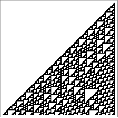
What we care about here is the initial condition. We can set the condition to be a periodic background:
Out[]=
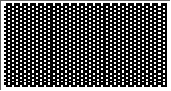
Let’s make things interesting now. We can “poke” the periodic background a bit, to create a perturbation. The results of the evolution then become more interesting:
Out[]=
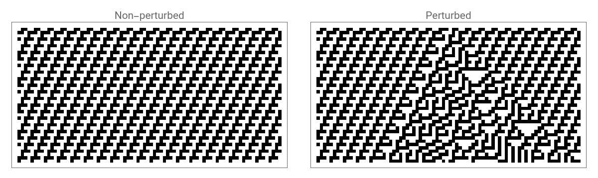
But there is another interesting way to make a perturbation, by clashing two periodic backgrounds so that their boundary acts as a perturbation:
Out[]=
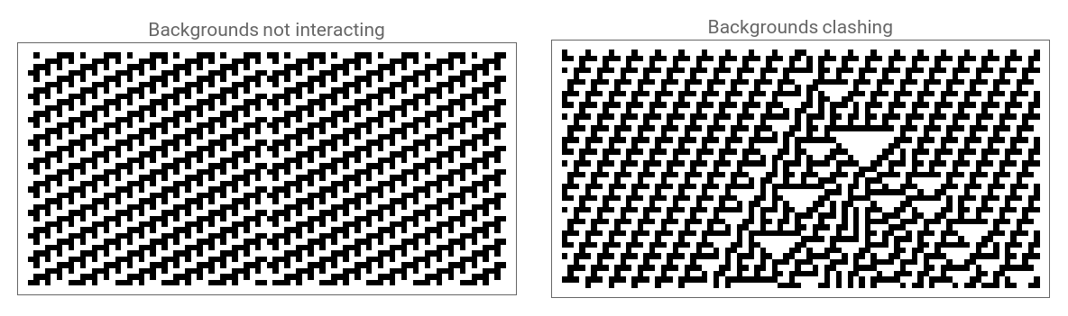
Let’s see how we can study and classify the propagation of these perturbations.
Perturbation in Periodic Background
Perturbation in Periodic Background
Generating the Evolution History
Generating the Evolution History
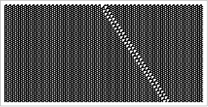
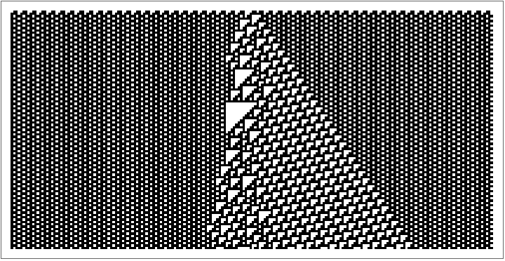
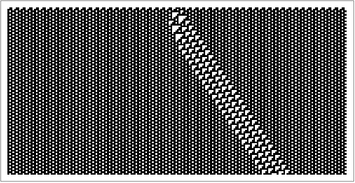
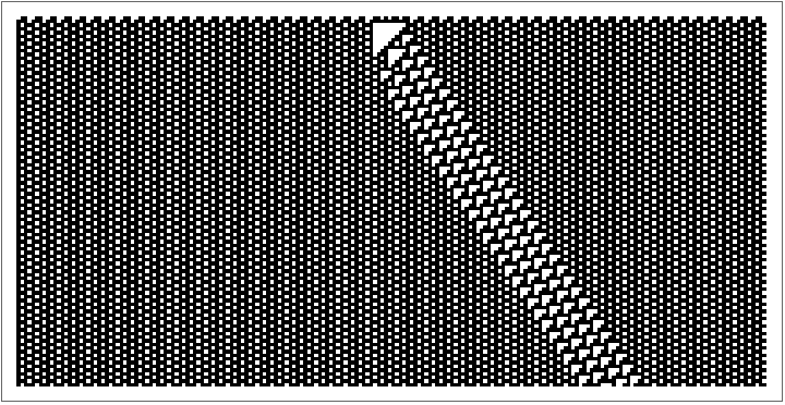
With the ultimate goal of classifying the perturbation behavior in mind, we will need to model its length over time. Let’s first generate the evolution of a cellular automaton, where the arguments are the rule, the background, the perturbation, and the number of steps. By generating a list of all the possible perturbations and backgrounds of a certain size, we can map the evolution history for multiple cases of arguments.
Here are some interesting cases for rule 110, with a background of {0, 1, 1, 0}.
Out[]=
,
,
,
,
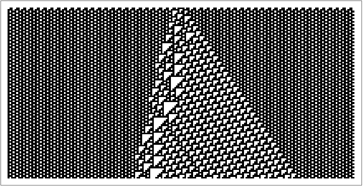
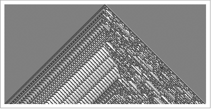
Here is a handy way to see the evolution for any rule with any perturbation and background pair, up to size 4.
Out[]=


Modeling the Perturbation Size
Modeling the Perturbation Size
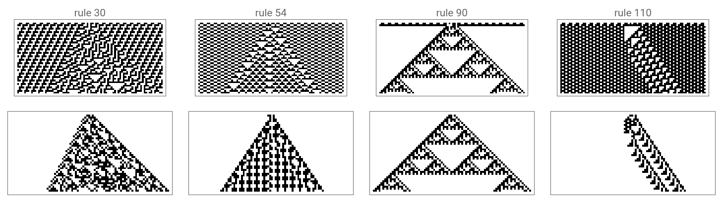
The perturbation size is modeled by taking the XOR between the unperturbed and the perturbed evolution for the respective arguments. Mapping for some exemplary rules, we can see the comparison of the length of the perturbation with the image of the evolution. Let’s demonstrate this comparison for two different step counts, with the background and perturbation being {0,1,1,0}, {1,0,1,1} respectively.
Out[]=
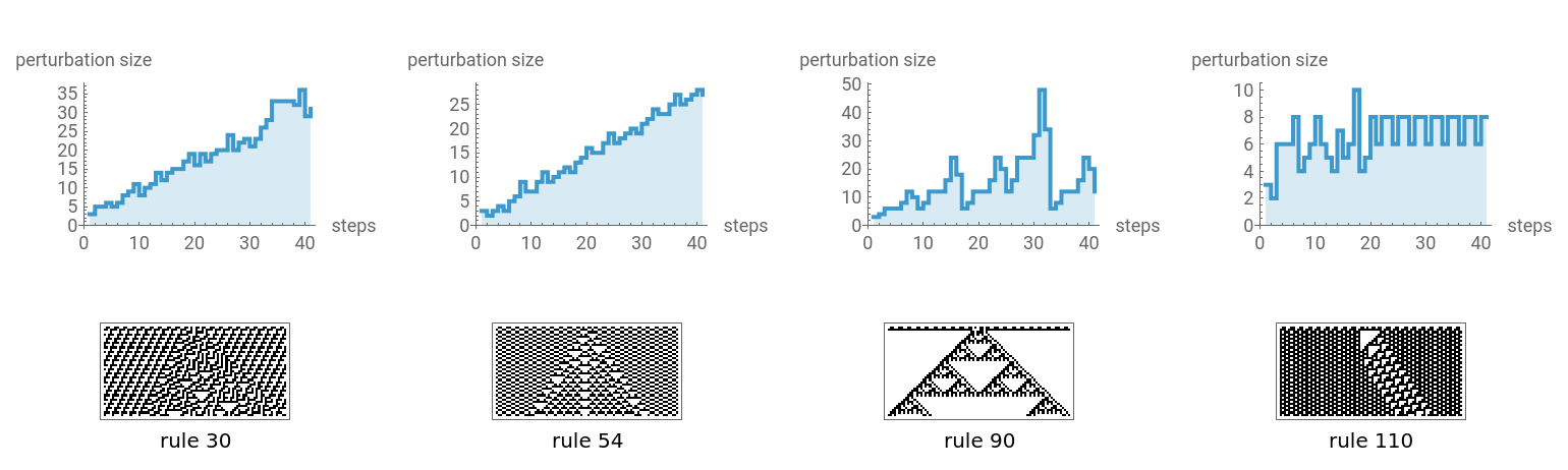
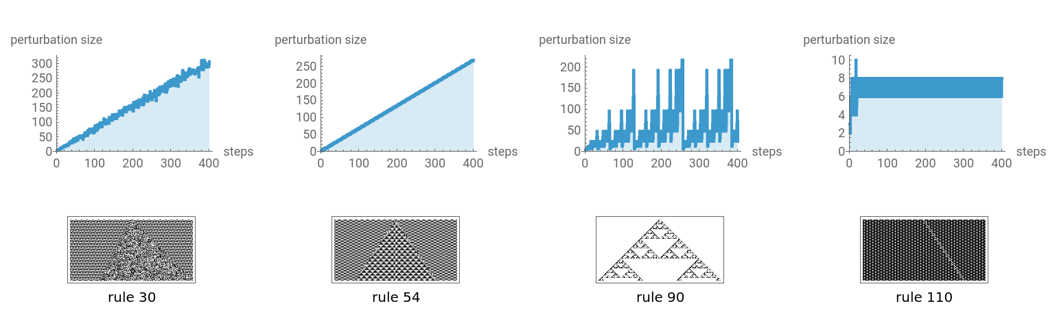
It is also possible to plot the perturbation by itself so we can clearly see how it evolves.
Out[]=
Finding Appropriate Backgrounds
Finding Appropriate Backgrounds
In the evolution of the perturbations, we can see that some backgrounds disappear after a number of steps. These backgrounds are not “appropriate” to be used for their respective rules. To fix this, we are going to use the nest graph of the evolution. The backgrounds that correspond to cycles in the nest graph (including self-loops) are the ones that do not disappear, and are allowed to use. Here are some examples of nest graphs for all the different backgrounds:
Out[]=
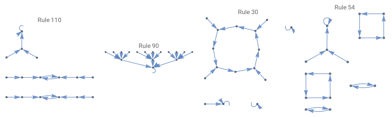
Let’s show the allowed backgrounds of rule 110, up to size 4, as an example:
Classifying the Behaviors
Classifying the Behaviors
To build a classification model, we first have to normalize the evolution. This means that we can rotate each step of the tape, and get an image like this:
If the maximum number of similar tapes in the normalized version is more than one, then it is repeating, and thus periodic. Let’s test that:
Sanity check: we saw earlier that the evolution of rule 54 is not periodic for these arguments, instead it seems to grow indefinitely.
Now we can make the classification model. According to the NKS, the classes of elementary cellular automata are Class 1, 2, 3, 4, in increasing order of complexity. We are going to build our classification model in a way that resonates with the NKS Class 1 classification.
◼
Class 1.1: Perturbations that disappear after a certain amount of steps.
◼
Class 1.2: Perturbations that stay periodic and don’t grow after a certain amount of steps.
◼
Class 1.3: Perturbations that are periodic but continue growing indefinitely.
In this project, we are going to classify classes 1.1 and 1.2. But there is a danger here: If a perturbation is classified as neither 1.1 or 1.2 in our model, that does not mean that it is class 1.3. A perturbation that is periodic could still start growing after many steps. So for these cases, instead of “Class 1.3”, the classification should return “Unknown Class”.
Let' s try it for one evolution as an example:
Let’s see a more explanatory representation of the perturbation length and each class:
It is also possible to classify all the possible perturbations for a certain rule and background:
Perturbation due to Background Clash
Perturbation due to Background Clash
As discussed in the introduction, the second type of perturbation that we are studying is that caused by the clash of two different periodic backgrounds during the evolution.
Primitive Backgrounds
Primitive Backgrounds
Some of these backgrounds represent the same background just with a different configuration.
For example, the background {0,1,0,1} is the same as the background {0,1}, so any cycle it belongs to at size 4 is already accounted for at size 2. A state is called primitive if it is not a repetition of a shorter block, or equivalently, if no rotation by a proper divisor of its length leaves it unchanged. Let’s eliminate these cases, and show only the primitive backgrounds:
For rule 110, all the backgrounds up to size 6 are the following:
All the backgrounds of size 4 are the following:
These are presented as matrices because this function also takes into account the period of these backgrounds in time. Below, we can see the period of one background both in time and in space, inside an evolution.
Now that we narrowed down the number of backgrounds, let’s make them fight.
Clashing the Backgrounds
Clashing the Backgrounds
Let’s see some interesting cases of primitive backgrounds interacting:
Rule 110:
Rule 30:
Rule 120 :
The interesting behavior here is shown by rule 120, which is a fairly non-famous rule. If we look at a typical evolution of rule 120 starting from a single black cell, it doesn’t initially look like much:
But when we evolve it with a clash of different backgrounds, the behavior is way more interesting. I would personally describe it as a “particle shower”.
For visualization purposes, we can choose a pair of backgrounds and show their collision for different rules:
Modeling the Perturbation Size
Modeling the Perturbation Size
In order to model the perturbation size like in the previous case, we will have to work differently because now we have two backgrounds instead of one. The model takes the difference between separate left and right background cases, and generates the length of the perturbation.
Here are some examples of the growths of a perturbation length for different rules and backgrounds:
Similar to before, there are some cases where the perturbations seem to grow indefinitely, and cases where they seem to stay periodic and don’t grow, like the third case where the length is oscillating between 1 and -2. In this case, Class 1.1 is impossible, since a perturbation caused by the boundary between the backgrounds cannot disappear.
Let’s see two examples of the classification:
Classifying the Behaviors
Classifying the Behaviors
In a similar manner as in the first case, what we want to do is classify these behaviors for different rules and background pairs.
For this model, we construct a function that figures out if a perturbation grows or not. Using this function, we can construct the classification model. Let’s try it:
We can also see the pairs of backgrounds that correspond to each class, for rule 110:
Future Work
Future Work
This project has a lot of potential for future work. There is an interesting technology which I was not quite ready to present yet, which manages to make a compressed evolution tape, in order to optimize the enumeration process in order to be able to classify more complex behaviors. As it is evident, this essay only focuses on classes up to 1.2, so a future scope would be to study perturbations that grow in a periodic, or chaotic way. Here is a sample of the output of the compressed tape technology:
{LBackground[{0,1,1,1},0,2],{0},RBackground[{0,1,1,1},0,0]}
Essentially the idea is to separate the tape into background and perturbation pieces, so any tape can be studied at any time of the evolution.
Another application of this research would be to find perturbations that move in opposite directions, and try to make them interact. The idea for this setup is to simulate particle collision behaviors. Furthermore, iterating the same idea into hypergraph-rewriting systems should produce interesting results.
Concluding Remarks
Concluding Remarks
This essay was an elementary approach to how particle behavior can be simulated through structures like cellular automata. Even though the correlation is at an elementary stage, this research was very interesting for me, despite the challenges. We were able to show how different perturbations behave in different settings, and model their size over time. Using this technology, we were able to build a framework that classifies different cases of behavior. An interesting extension would be to enumerate many cases using the ClassEvolution function, and create a statistical analysis of the frequency of each class for different rules. Overall, this research program has been extremely interesting for me, and has exposed me to new computational methods and opportunities. I believe that this research can serve as a basis for future work that will yield interesting results.
Perturbation in Periodic Background Code
Perturbation in Periodic Background Code
Acknowledgments
Acknowledgments
I would like to thank my mentor, Max Piskunov, for his help, ideas, and suggestions throughout this project. A special thank you to Stephen Wolfram for providing both the idea and the outline for the first steps of this research project. I am also grateful to all the other mentors and teaching assistants that helped me with coding and intellectual challenges during this project. Lastly, I want to thank all my friends in this program for their constant support.
References
References
1
.Stephen Wolfram (2002), A New Kind of Science. Wolfram Media.
2
.Stephen Wolfram (2020), A Class of Models with the Potential to Represent Fundamental Physics. https://www.wolframphysics.org/technical-introduction/
3
.Matthew Cook (2004), Universality in Elementary Cellular Automata, Complex Systems.
4
.Stephen Wolfram (1984), Universality and Complexity in Cellular Automata, Physica D: Nonlinear Phenomena.
AI Disclosure
AI Disclosure
The following generative AI tools were used in this project: Claude Fable 5 was used for constructing one of the functions in the code. All code and written content was reviewed, understood and approved by the author.
CITE THIS NOTEBOOK
CITE THIS NOTEBOOK
Classifying Defects in Cellular Automata
by Myrto Terpsiadou
Wolfram Community, STAFF PICKS, July 16, 2026
https://community.wolfram.com/groups/-/m/t/3761646
by Myrto Terpsiadou
Wolfram Community, STAFF PICKS, July 16, 2026
https://community.wolfram.com/groups/-/m/t/3761646