We study the Feynman checkerboard model in (1+1)-dimensional spacetime. The Kac model, a classical equivalent of the Feynman checkerboard, is also discussed. A graph theoretic approach to these models is developed and applied to different spacetime graphs.
Walks on a rectangular (1+1)-lattice
Walks on a rectangular (1+1)-lattice
The Kac Model
The Kac Model
Firstly, we consider the classical analogue of Feynman’s checkerboard, which is known as Kac’s model [1]. In a (1+1)-dimensional spacetime, Kac’s model describes a particle whose allowed positions fall on an equidistant lattice
Out[]=

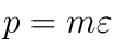
where is the position and is the grid spacing. Time, , is also discretized in units of (the full spacetime lattice is then ). The velocity of the particle is ±1 and may switch direction with probability on each time-step. By passing to the continuum, the probability density, , associated with finding the particle at spacetime point evolves like




Out[]=

which is a so-called “telegraph” equation [1, 2]. By modifying , the telegraph equation may be written

Out[]=

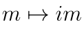
which reproduces the Klein-Gordon equation as [2]. We simulate the Kac model in a later section of this notebook.
The Feynman Checkerboard
The Feynman Checkerboard
The Feynman checkerboard is similar to the Kac model in its basic setup. The particle is again constrained to occupy sites on the lattice. Motion of the particle is along light-like edges connecting lattice sites. However, instead of tracking the probability at each cell, the basic Feynman checkerboard model assigns to every cell a -number, representing the amplitude for propagation to that cell. The amplitude is calculated using a “sum over paths” technique [3]

Out[]=

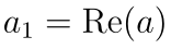
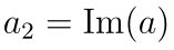
where is any path connecting the initial spacetime point and . Up to an overall normalisation (which is constant across all paths with space-like separated termination points), the amplitude for a specific path is set by the number of turns in that path. Assigning a complex phase to the state packages quantum phenomena (e.g. interference) into the checkerboard model.By decomposing the amplitudes into their real and imaginary parts, and , one can write update equations [3] akin to cellular automaton rules

Out[]=

Out[]=

which reduce to a Dirac-like equation in the limit

Out[]=

Indeed, in the continuum limit
Out[]=

Out[]=

where is the order Bessel function of the first kind. Moreover, the retarded propagator is found to be

th
n
Out[]=

which is in agreement with standard QED [3]. Outstanding questions are whether Feynman’s checkerboard remains a valid algorithmic approach to QED when extended to 3+1 dimensions or when modelled with interactions.
Implementing Feynman’s checkerboard
Implementing Feynman’s checkerboard
A straightforward implementation of the “sum over paths” technique can be used to calculate amplitudes for an electron propagating in 1+1 spacetime. In Figure 1, time runs downwards with space on the horizontal. For the amplitude plots, the colour is related to the argument of the local amplitude; opacity is related to modulus of the amplitude.
Out[]=

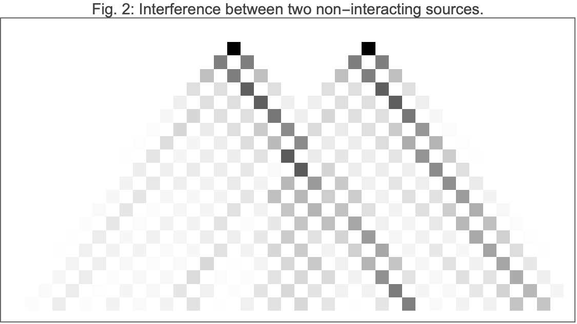
By adding another source, we can study interference effects. Figure 2 shows the resultant probabilities for two non-interacting electrons.
Out[]=
A graph theoretic approach to arbitrary lattices
A graph theoretic approach to arbitrary lattices
Preliminaries
Preliminaries
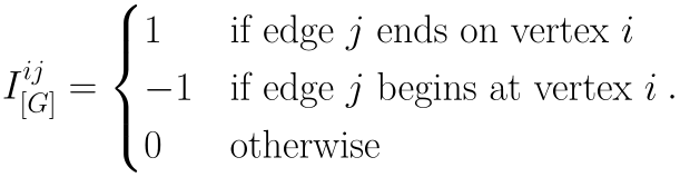
There is some uncertainty in the literature how to consistently extend the checkerboard model from 1+1 to 3+1 spacetime. Inspired by [4, 5, 6], we develop an approach which might work on arbitrary spacetime topologies. By representing spacetime as a graph, we use the incidence matrix to construct evolution operators which evolve quantum states on the graph. If the (1+1)-Feynman checkerboard can be recovered in this approach, the (3+1)-dimensional case is obtained by changing the topology of the underlying spacetime graph.The incidence matrix of a digraph is defined [4, 7]

Out[]=
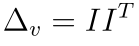
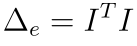
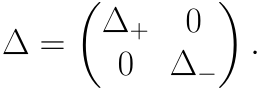
Using the incidence matrix, we can define a vertex Laplacian and an edge Laplacian . With and there are two kinds of walk which can be simulated on an arbitrary graph. Firstly, the quantum state might be specified by assigning -numbers to each node of the spacetime graph. In this case, iterating on the state simulates a vertex-to-vertex walk of the system. Otherwise, by specifying -numbers on each edge and iterating with , we simulate an edge-to-edge walk of the system. The Hodge Laplacian, , is the block-diagonalisation of and


Out[]=
Unitary time evolution of the state is implemented by the Schrodinger-like equation [4]
Out[]=
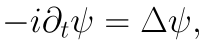
where is a vector in , with n being the total number of vertices and edges in the graph. To implement Dirac-like evolution, we define a “Dirac operator” as a formal ‘square root’ of the Laplacian [4]


Out[]=
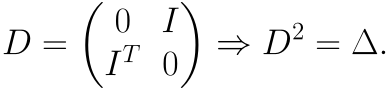
A single iteration of the Dirac operator evolves the state by a ‘half-step’; the state is moved forward by a single vertex-to-edge or edge-to-vertex step. In this case, the state evolves according to a Dirac-like equation [4]
Out[]=

If the graph is foliated into space-like subgraphs, one should be careful to appropriately remove negative entries from the incidence matrix. Otherwise, particles may “back propagate” along directed edges instead of moving uniformly “forward” in time.
In the Kac Model
In the Kac Model
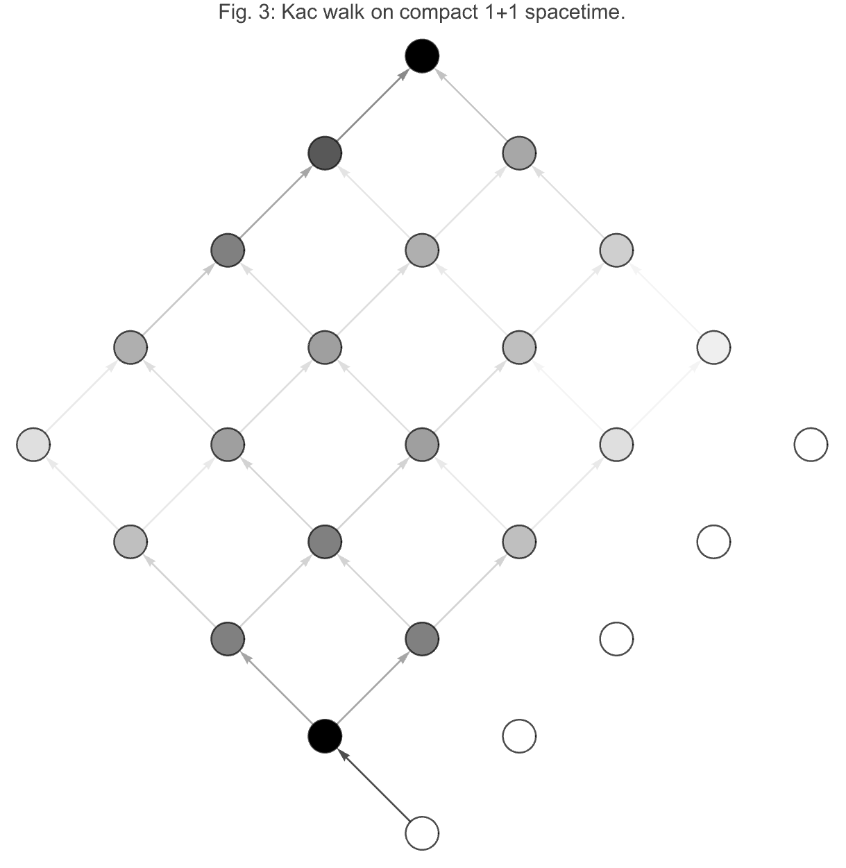
As a first example, we treat a classical walk on a compact (1+1)-dimensional spacetime. In Figure 3, we show the probability that an initially left-moving particle propagates to various cells. In the embedding of Figure 3, each row corresponds to a different space-like foliation, with time increasing upwards.
Out[]=
To illustrate the versatility of the graph-theoretic method presented here, we show the same classical walk on a toroidal spacetime in Figure 4.
Figure 5 shows that we can also calculate Kac walks on spacetimes with holes punched in them.
In the Checkerboard Model
In the Checkerboard Model
Unlike the Kac model, the “observable” being tracked in each ‘Feynman checker’ is not a probability but rather the (complex) amplitude for propagation to that cell (which recovers the probability after mod-squaring). In this approach, we update a state defined on just the edges of the spacetime graph. The amplitude is computed by assigning phases to edges leading into or out of a given vertex and summing over the resulting edge weights.
Rectangular lattice
Rectangular lattice
In Figure 6, our technique is applied to the same rectangular 1+1 spacetime studied in Figure 1. We obtain compatible results for the electron amplitudes. The colour and opacity of each cell is related to the argument and modulus of the local amplitude. The colour and opacity of the edges are related to the sign and magnitude of the local edge weight.
Toroidal lattice
Toroidal lattice
Our graph theoretic approach remains robust on non-standard grids. Figure 7 shows amplitudes calculated on a toroidal spacetime. The same colouring scheme is used as in Figure 6.
Concluding Remarks and Future Work
Concluding Remarks and Future Work
The work presented in this notebook is a proof-of-concept for the use of graph theoretic techniques in computing Feynman checkers. Imminent extensions to our model include 3+1 and curved spacetimes.
Acknowledgments
Acknowledgments
I sincerely thank Nikolay Murzin and Nicholas Frieler for their excellent mentorship. Nikolay and Nicholas both provided help with coding, with Nikolay also kindly discussing physics with me. The idea for this project is due to Stephen Wolfram and is based on previous work by Nikolay Murzin.
References
References
1
.M. Kac (1974), “A Stochastic Model Related to the Telegrapher’s Equation”, Rocky Mountain Journal of Mathematics. https://www.jstor.org/stable/44236399
2
.G.N. Ord (2023), “The Feynman Chessboard Model in 3+1 Dimensions”, Frontiers in Physics. https://www.frontiersin.org/journals/physics/articles/10.3389/fphy.2023.1286030/full
3
.M. Skopenkov and A. Ustinov (2020), “Feynman Checkers: Towards Algorithmic Quantum Theory”. https://arxiv.org/abs/2007.12879
4
.B. Casiday et al. (2024), “Laplace and Dirac Operators on Graphs”, Linear and Multilinear Algebra. https://www.tandfonline.com/doi/abs/10.1080/03081087.2022.2158297
5
.N. Delporte et al. (2024), “Dirac Walks on Regular Trees”, Journal of Physics A: Mathematical and Theoretical. https://iopscience.iop.org/article/10.1088/1751-8121/ad4d2e/meta
6
.G. Bianconi (2024), “The Mass of Simple and Higher-Order Networks”, Journal of Physics A: Mathematical and Theoretical. https://iopscience.iop.org/article/10.1088/1751-8121/ad0fb5/meta
7
.M. Van Steen (2010), Graph Theory and Complex Networks: An Introduction. M. Van Steen.
8
.E.M. Lifshitz et al. (1989), Quantum Electrodynamics. Elsevier Science.
9
.G.N. Ord and E. Harley (2009), “Numerical Experiments in Relativistic Phase Generation through Time Reversal”, Advanced Studies in Theoretical Physics. https://www.m-hikari.com/astp/astp2009/astp1-4-2009/ordASTP1-4-2009.pdf
10
.L.H. Kauffman and H. Pierre Noyes (1996), “Discrete Physics and the Dirac Equation”, Physics Letters A. https://www.sciencedirect.com/science/article/abs/pii/0375960196004367
11
.P. Arrighi (2019), “An Overview of Quantum Cellular Automata”, Natural Computing. https://link.springer.com/article/10.1007/s11047-019-09762-6
Boilerplate
Boilerplate
Cite This Notebook
Cite This Notebook
“A Graph Theoretic Approach to Feynman Checkers”
by Gary G. Louw
Wolfram Community, 9 July 2025
https://community.wolfram.com/groups/-/m/t/3497586?p_p_auth=jF3J4MQ6
by Gary G. Louw
Wolfram Community, 9 July 2025
https://community.wolfram.com/groups/-/m/t/3497586?p_p_auth=jF3J4MQ6