In the Wolfram Physics Project, space is thought of as hypergraph where the only information we have are relations between vertices. This hypergraph evolves by changing via rules applied to it. The application of a rule is called an event so we can create a causal graph that shows the causation between different events. We can analyze these causal graphs by looking at a graphon which is essentially a colored adjacency matrix. In these causal graphons, different structures form but the most prominent ones are lines. We analyze these lines and see how they are related to physics -- specifically, we find that the slope of the lines give us the speed of light in the universe described by the rule.
Initialization
Initialization
Introduction
Introduction
In the Wolfram Physics Project, space is thought of as a discrete set of points connected by hyperedges which are edges that can connect multiple vertices. These hypergraphs based on rules like this
Out[]=

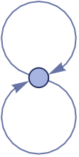
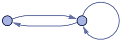
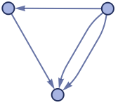
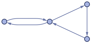
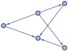
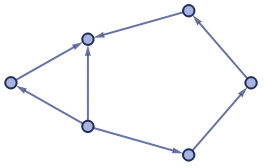
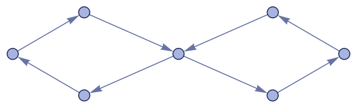
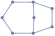
This means that we look through the current state of the hypergraph for the pattern on the left and change it to the pattern on the right. We can look at the evolution of a hypergraph as we do this process stating from the initial condition and for the rule above, we get the following evolution:
Out[]=
,
,
,
,
,
,
,
,
,
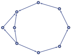
,
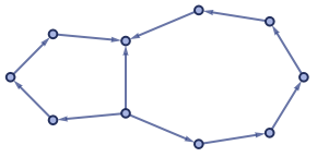
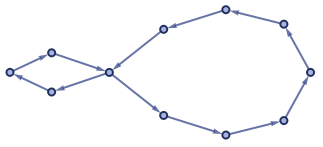
We can change the hypergraphs in different orders and these events depend on each other so we can construct a causal graph. For the last step of the previous example, the causal graph would be:
Out[]=
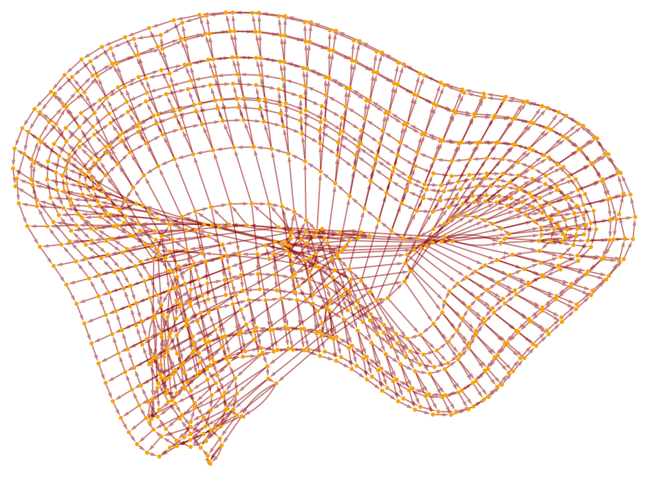
One way to analyze this graph is to use graphons.
What are graphons?
What are graphons?
Consider a 10-vertex undirected graph where two vertices are connected with probability 1/2. The adjacency matrix looks like this:
Out[]=
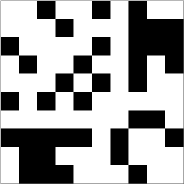
where 1 → black and 0 → white. If we increase the number of vertices, we get,
Out[]=
,
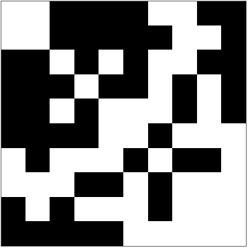
,
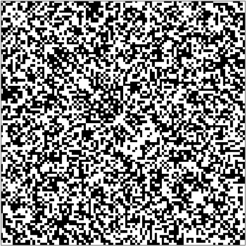
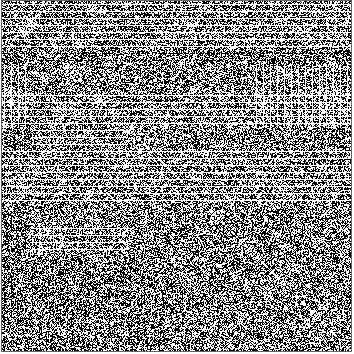
This eventually becomes this:
Out[]=

Notice that as we increase the number of vertices the square becomes uniformly filled with a gray halfway between white and black which represents 1/2. Therefore, the graphon of this graph is the constant function that sends points in to 1/2. In general, a graphon is a function from where for a pair of vertices consider and and let be the number of edges between and (Han). Here’s another example:
2
[0,1]
W:[0,1]
2
[0,1]
(j,k)
x∈[(j-1)/n,j/n]
y∈[(k-1)/n,k/n]
W(x,y)
j
k
In[]:=
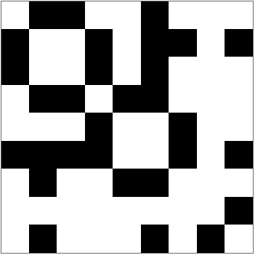
Table[edges={};Table[Table[If[RandomReal[]<=1-i/c,AppendTo[edges,{j,i}]],{j,i-1}],{i,c}];ArrayPlot[AdjacencyMatrix@Graph[edges],ImageSize->Small],{c,{10,100,500}}]
Out[]=
,
,
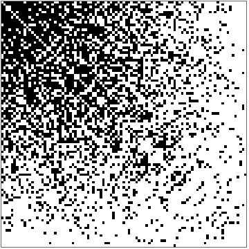
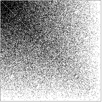
As we add more vertices, the probability of adding edges goes down linearly.
In this project, we use graphons to study large scale structures like above, we can see vertices in the top left are more connected than other vertices. From now on, we when talk about graphons we mean graphons where the the number of vertices goes to infinity.
In this project, we use graphons to study large scale structures like above, we can see vertices in the top left are more connected than other vertices. From now on, we when talk about graphons we mean graphons where the the number of vertices goes to infinity.
Edge Density
Edge Density
We can extract different features of a graph from its graphon like its edge density which tells us what fraction of the maximal number of edges a graph has. This is the same as the average degree of the vertices divided by the number of vertices so the edge density is . Essentially, we are integrating the graphon over .If we do this for the first graphon we just get 1/2 since the graphon is . Oftentimes, we don't have a closed form for the graphon so we can approximate the edge density with a graphon of finite vertices. In this case, we use 500 vertices:
∫∫W(x,y)dxdy
2
[0,1]
W(x,y)1/2
We first find possible edges in "allEdges" for a 500-vertex graph. Then we add an edge to our graph with probability 1/2 and find the adjacency matrix. We sum everything in the matrix and multiply by 1/500^2 since the dimension of the adjacency matrix is 500 x 500.
In[]:=
allEdges=Flatten[Table[Table[{i,j},{j,i+1,500}],{i,500}],1];g=Graph@Select[Table[If[RandomInteger[]==1,i],{i,allEdges}],ListQ];N[Total[Total[AdjacencyMatrix@g]]/(500^2)]
Out[]=
0.497928
This makes sense since out of the maximal number of the edges, half of them will actually exist since the probability of an edge existing is 1/2.
The second graphon is a good example of need to approximate the double integral since the closed form is not the nicest to integrate:
The second graphon is a good example of need to approximate the double integral since the closed form is not the nicest to integrate:
We increase the number of vertices from 10 to 100 to 500 and integrate the graphon.
In[]:=
edges={};Table[Table[Table[If[RandomReal[]<=1-i/k,AppendTo[edges,{j,i}]],{j,i-1}],{i,k}];N[Total[Total[AdjacencyMatrix@Graph[edges]]]/(k^2)],{k,{10,100,500}}]
Out[]=
{0.22,0.3244,0.34484}
Causal Graphons
Causal Graphons
Recall the causal graph from before which had this rule:
Out[]=
The graphon of this is
In[]:=
ListAnimate[Table[ArrayPlot[ResourceFunction["WolframModel"][{{x,y},{x,z}}->{{y,w},{y,z},{w,x}},{{0,0},{0,0}},i,"CausalGraph"]//AdjacencyMatrix,ImageSize->Medium],{i,1,1000,10}]]
Out[]=

Notice the line in the middle and perpendicular lines. It is important to note that the middle line is not actually the center diagonal line and is shifted to the right by one pixel. This has to be the case since events do not cause each other. Let us zoom in to see what these structures say about the causal graph.
However, after the 16th timestep, these diagonals start breaking down. Above is the graphon after 40 time steps.
When we calculate the edge density for this graphon for different number of vertices, we get:
Notice that the edge density goes to 0 indicating that the causal graph is sparse. This makes sense since lots of events will not be connected to each other. This is because there is a natural flow of events and events lower in the flow don't cause events upper in the flow.
Here are other causal graphons of other rules
Most of these rules produce lines but here is a weird rule that produces a curve:
For all 16 rules of this signature, the causal graphs are identical so they all produce the same graphon which is just a line with the following slope:
Here are two rules with this signature
Finding Clusters in the Graphons
Finding Clusters in the Graphons
This basically looks at features in the graphons and puts graphons with similar features close to each other.
Here is the code for the plot above but this takes a very long time to run.
Here are 100 graphons that are already evaluated.
Interpretation of the Structures in Causal Graphons
Interpretation of the Structures in Causal Graphons
Consider the following rule
with the following graphon
The causal graph is
which is just a chain of events.
In a lot of these rules including the one above, there are lines in the graphons so an obvious question is: what do these lines mean? In the rule above, the line through the center of slope -1 indicates that on average, each vertex is connected to exactly one vertex. However if we consider the following rule:
In a lot of these rules including the one above, there are lines in the graphons so an obvious question is: what do these lines mean? In the rule above, the line through the center of slope -1 indicates that on average, each vertex is connected to exactly one vertex. However if we consider the following rule:
with the following graphon
it has a line with a slope of smaller magnitude. We can extract the slope of the line with,
This means that 49% of the vertices are connected to another vertex so on average each vertex is connected to 1/0.493921 = 2.02 vertices. Therefore, the causal graph grows faster for this rule than the first and sure enough, we have,
From the point of view of physics, a causal graph is the analog of a light cone i.e. starting from one vertex, the vertices we can reach is analogous to the points in spacetime light can reach. This means that a faster growing causal graphs have a faster speed of light and we just found that causal graphs grow faster the flatter the line in the graphon is. Therefore, the slopes of the lines in the graphons represent the speed of light.
In some of the other rules above there were multiple lines and we speculate that in these universes the speed of light is not constant and different lines represents different reference frames.
In some of the other rules above there were multiple lines and we speculate that in these universes the speed of light is not constant and different lines represents different reference frames.
Conclusions
Conclusions
Overall, one way to visualize causal graphs are with graphons which are colored adjacency matrices. These graphons can form interesting and surprisingly regular structures like lines and curves. These structures can tell us various things about the causal graph like how fast it grows which can then tell us about properties of the universe the rule describes. Specifically, the slope of the line in the graphon represents the speed of light. We can also look at similarities in features of graphons and cluster them by these similarities.
Some future work could be clustering more graphons. In this work, we were able to plot only 100 graphons since computing causal graphs to the level of resolution we needed to took a lot of time but more defined clusters could form if we have more graphons. Additionally, we have only looked at a very small slice of the total number of rules (in fact an infinitesimal slice) so in the future, we could look at more rules to see if other interesting structures form in the causal graphons.
Some future work could be clustering more graphons. In this work, we were able to plot only 100 graphons since computing causal graphs to the level of resolution we needed to took a lot of time but more defined clusters could form if we have more graphons. Additionally, we have only looked at a very small slice of the total number of rules (in fact an infinitesimal slice) so in the future, we could look at more rules to see if other interesting structures form in the causal graphons.
References
References
◼
Han, Valerie. The Graphon as a Limit for Dense Graphs. https://math.uchicago.edu/~may/REU2018/REUPapers/Han.pdf
◼
Glasscock, Daniel. WHAT IS ... a Graphon? https://arxiv.org/pdf/1611.00718.pdf
Acknowledgements
Acknowledgements
I would like to thank Jeremy Stratton-Smith for his patience and help understanding the concepts behind this project.
CITE THIS NOTEBOOK
CITE THIS NOTEBOOK
Analyzing structures in causal graphons and potential applications to fundamental physics
by Nandana Madhukara
Wolfram Community, STAFF PICKS, July 13, 2023
https://community.wolfram.com/groups/-/m/t/2964917
by Nandana Madhukara
Wolfram Community, STAFF PICKS, July 13, 2023
https://community.wolfram.com/groups/-/m/t/2964917