My project begins with the central question: Can we analyze model performance by using ranking models and dimensionality reduction to uncover hidden insights? We’re exploring how LLMs handle math and logic questions of varying complexity. The dataset compares each model’s output directly against the ground truth. Our goal is to analyze patterns in how and where models succeed or struggle and to visualize those patterns, and gain insights into model outputs through computational exploration.
Overview
Overview
Introduction
Introduction
As LLMs continue to evolve from base models to instruction-tuned assistants and conversational agents, they are increasingly evaluated based on simple accuracy metrics or subjective qualitative assessments. However, these approaches often overlook how different models behave across the same standardized set of problems and whether their correctness patterns encode deeper, more meaningful behavior.
This project aims to fill that gap by analyzing a large dataset containing binary correctness responses from 461 LLMs evaluated on 671 math and logic questions. The models span a wide range, from smaller, instruction-tuned models to famous chatbots like GPT-4, Claude 3.5,.
By applying methods such as dimensionality reduction, Bradley-Terry scoring, and visual exploration techniques, we seek to understand:
◼
Which models consistently outperform others?
◼
Which questions are universally difficult?
◼
Are performance trends correlated with cost, recency, or vocabulary complexity?
We aim to present both intuitive visual stories and robust quantitative evidence about the landscape of models.
Dataset Overview
Dataset Overview
The dataset comprises binary correctness scores for a set of questions answered by multiple LLMs across a wide set of mathematical and general knowledge questions.
Read the dataset:
Examples: Below are a few example entries from the dataset to understand its structure and content:
Dimensionality Reduction of Model Responses
Dimensionality Reduction of Model Responses
Understanding LLM behavior across hundreds of questions involves working with high-dimensional data, where each model is represented by a binary correctness vector spanning 676 dimensions. To visualize this landscape, we employ Principal Component Analysis (PCA), a standard dimensionality reduction technique that preserves the most significant variance in the data while reducing it to a 2D space.
What is PCA, and Why Use It?
Principal Component Analysis is a linear transformation technique that projects high-dimensional data onto a lower-dimensional subspace, where each new axis (principal component) captures as much of the original data' s variance as possible. In this context, PCA enables us to identify clusters of models with similar performance patterns without the need to inspect all 676 dimensions manually.
Additionally, we stick with PCA here, not only for simplicity, but also because we will later validate this choice using a scree plot.
Visualizing models in 2 D allows us to see how they group, overlap, or separate based on shared patterns of correctness across questions. Clusters often correspond to similar model families or training objectives.
Module{models,points,overallPerformance,colors,cfName="RedBlueTones"},models=Keys[allModelQuestions];overallPerformance=Values[ReplaceAll[Total@*DeleteMissing@*Values/@allModelQuestions,{True->1,False->0}]];colors=Map[ColorData[cfName],Rescale[N[#],MinMax[#]]&@overallPerformance];points=DimensionReduce[Values@Replace[Values/@allModelQuestions,{True->1,False->0},{2}],2,Method->"PrincipalComponentsAnalysis"];ListPlotAssociationThread[Style[#,Small]&/@models,MapThread[Style[#1,#2]&,{points,colors}]],
Out[]=
|
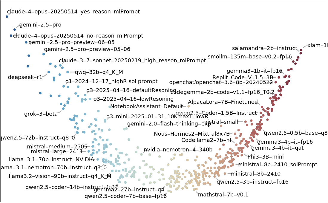

This plot (above) reveals an interesting pattern: most models align along a narrow curved band in the 2D PCA space. This suggests a substantial one-dimensional variation in performance across the benchmark. In other words, despite architectural or training differences, the dominant trend is the overall accuracy of a model in answering questions correctly. In the next section, we’ll validate this observation with a scree plot, which helps confirm how much of the variance is truly captured by the first component.
Out[]=
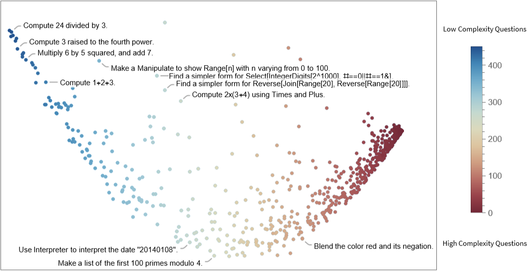
This plot (above) shows how questions relate to each other based on the consistency of model responses. Compared to the model projection, we observe slightly more spread, but the dominant variation still lies along a single dimension. This suggests that most questions are not widely spread, as the dataset focuses on only a few topics.
Bradley–Terry Models for Scoring Models and Questions
Bradley–Terry Models for Scoring Models and Questions
While PCA gives us a visual sense of how models and questions behave in aggregate, it doesn’t directly provide quantitative view. To address this, we apply the Bradley-Terry model, a statistical method for estimating the relative “performance” of entities based on pairwise comparisons.
What is the Bradley-Terry Model?
◼
Each model is viewed as a “player” competing against other models on a set of shared questions.
◼
If a model gets a question right while another gets it wrong, that counts as a “win”.
◼
This approach yields a single score for each model, reflecting how often it outperforms other models.
◼
The same logic can be applied to score questions based on how often they “beat” models.
We construct a pairwise comparison matrix from the model-question correctness data and apply iterative updates based on the Bradley-Terry algorithm.
Bradley-Terry Modeling CodeText
Bradley-Terry Modeling CodeText
Model Scores
Model Scores
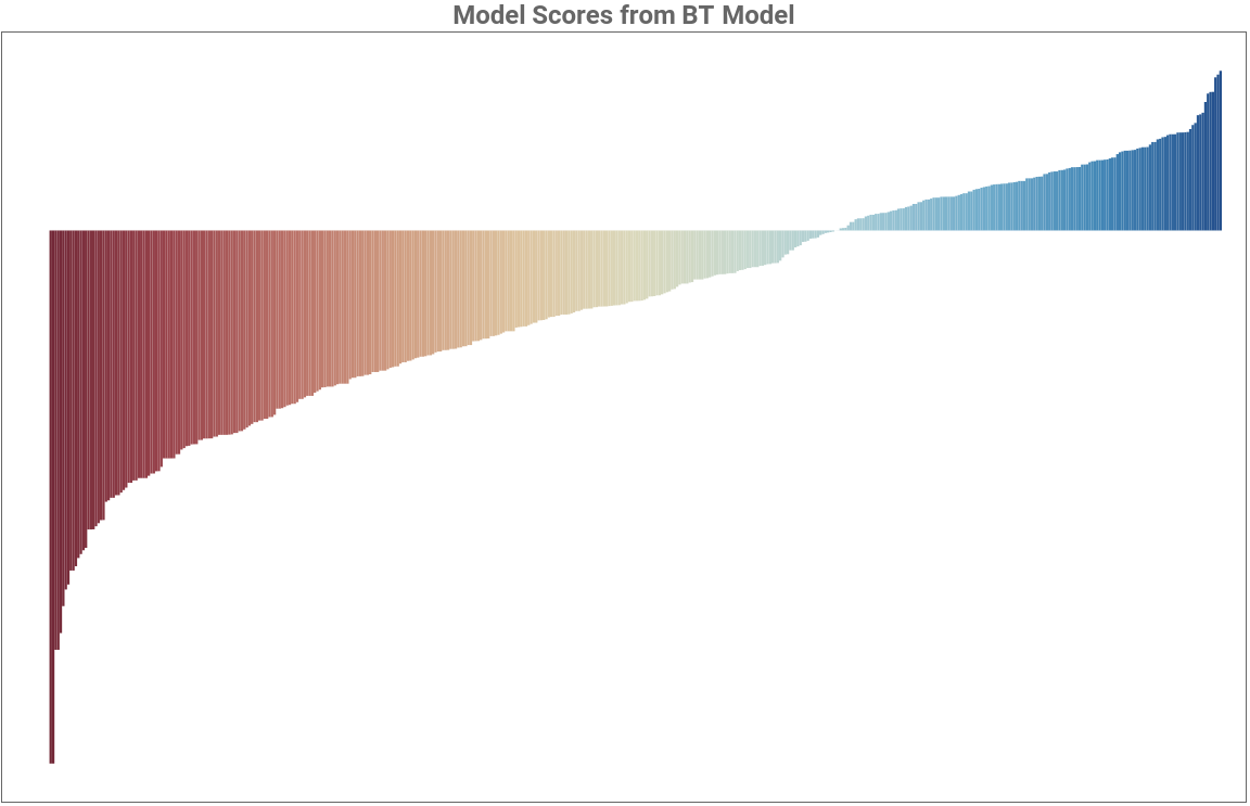
The following bar chart presents sorted model scores (on a log scale), providing a high-level view of how LLMs rank relative to each other across the benchmark.
Out[]=
Out[]=
|
|
Question Scores
Question Scores
Scree Plot Analysis: Justifying ONE Dimensionality
Scree Plot Analysis: Justifying ONE Dimensionality
In the first section, we saw that most models followed a nearly one-dimensional trend in the PCA space. To validate this observation, we use scree plots-a standard diagnostic tool in PCA. A scree plot shows the proportion of variance explained by each principal component. A steep drop after the first few components typically suggests that most of the variation is captured in just a few dimensions.
Observation:
Observation:
◼
For models, we observe a steep drop after the first component, confirming our earlier interpretation: most of the performance variation across models is explained by a single latent factor.
◼
For questions, we also see a strong first component. However, the decay is slightly more gradual, indicating that while a large portion of question behavior is multidimensional (difficulty), there may be a few additional dimensions capturing subtler patterns.
Visualizing Score Distributions and Predictability Patterns
Visualizing Score Distributions and Predictability Patterns
2. This histogram visualizes the predicted probability (from the Bradley-Terry model) that a model answers a question correctly, split into actual correct and incorrect attempts.
3. We narrow our focus to the top 50 models.
4. To quantify this, the overall predictive accuracy is ~0.80. For the top 50 models, it increases to ~0.86, confirming the quality of our scoring method.
◼
Predictability is highest for both straightforward and challenging questions.
◼
Predictability drops for questions of moderate difficulty, indicating more variability in model correctness.
◼
Interestingly, stronger models are more complex to predict.
◼
This could indicate that high-performing models make fewer mistakes, but those mistakes are not easily explained or anticipated.
Visualizing Cost vs Performance of LLMs
Visualizing Cost vs Performance of LLMs
We start by joining model capability scores (from the Bradley-Terry model) with cost metadata (input + output token costs). Next, we compute performance per dollar, which allows a fair comparison across models with different pricing schemes:
We use a log-log scale because both cost and score span orders of magnitude. This reveals relative efficiency rather than absolute values.
Observation:
Observation:
◼
Performance increases with cost, but not in a linear manner. You’ ll notice that low-cost models have a large spread (some perform poorly, some punch above their price); High-cost models generally achieve higher scores, but diminishing returns kick in.
Visualizing Release Dates vs Performance of LLMs
Visualizing Release Dates vs Performance of LLMs
Analyzing the Impact of Vocabulary Prompts
Analyzing the Impact of Vocabulary Prompts
The performance of models is nearly identical whether or not vocabulary support is included. The data points lie close to the diagonal line, indicating minimal difference across the models.
2. To fairly compare the same question prompts, we first remove the vocabulary prefix:
Conclusion
Conclusion
We revealed several interesting insights:
◼
Dimensionality reduction techniques revealed clusters of models, despite often aligning with shared architectures or tuning strategies.
◼
While more expensive models generally outperform cheaper ones, the performance gap is not strictly linear.
◼
Model performance has improved over time, but not dramatically. The most recent models show incremental gains, highlighting that newer does not always mean significantly better.
◼
Interestingly, including vocabulary prompts in questions did not consistently lead to improvements in accuracy. In many cases, stripped-down questions performed as well as, or even better than, their full-length counterparts.
Limitations
Limitations
While this analysis offers interesting insights into model behavior, it also has certain limitations. The dataset is restricted to logic and math questions, which may not fully represent the broad spectrum of tasks LLMs are capable of. Additionally, the binary correctness labels (1/0) offer a simplified measure of performance and may miss nuances in model responses.
Another key constraint is the computational cost limitations, we cannot easily rerun or expand these evaluations, this limits deeper longitudinal analysis or broader generalization beyond the current sample.
Another key constraint is the computational cost limitations, we cannot easily rerun or expand these evaluations, this limits deeper longitudinal analysis or broader generalization beyond the current sample.
Future Work
Future Work
As new models are released, this notebook can be updated to incorporate their performance data, enabling ongoing benchmarking. An inspiring direction would be to explore cross-linguistic evaluation: how does model accuracy shift when the same problem is posed in different languages and paraphrasing?
I extend my special appreciation to my mentor, Christopher Wolfram. His guidance has been exceptional, and he is undoubtedly one of the most talented individuals I have had the privilege to learn from. Thank you for the bouldering sessions and all our random talks!
I would also like to offer a profound acknowledgment to Piero Sanchez, John McNally, and Daniel Scarvalho for their invaluable support, and Stephen Wolfram himself, for his guidance.
References
References
Cite This Notebook
Cite This Notebook