In this project, I studied the value representing the number of elements of a discrete ball in a lattice L. We first find some polynomials that represent the general formula of in 2-dimensions for lattices that correspond to regular tilings of the plane. Then, using a general formula to obtain the d-dimensional analog of a 2D lattice, I calculated the formula for in d-dimensions using Ehrhart theory and generating functions. I then generalized the result to periodic graphs in reference to a paper by Inoue and Nakamura. From then on, I used the method of magnitude homology to explore more details on and some of its properties. Additionally, I also obtained a formula that creates a relationship between the cycles on the graph of and the number .
||
V
r
||
V
r
||
V
r
||
V
r
||
V
r
||
V
r
Introduction
Introduction
In the Wolfram Physics Project, there has been many efforts into attempts at creating a physical theory using hypergraphs. Indeed, a component to the theory is the notion of dimension in a hypergraph. Consider a ball in a hypergraph with geodesic metric. Then a reasonable assumption to prove is that the rate in which the number of elements in such a graph increases when the radius r increases is proportional to , where d is the dimension the hypergraph is embedded in. In this paper, I will show that that assumption is true not in just hypergraphs but in periodic graphs as well. Additionally, I will provide more insight into some topological properties to .
d
r
V
r
Cubical Case
Cubical Case
In geometry, there is an intimate relationship between the dimension a certain shape is and its volume. Consider the following grids that correspond to , , and respectively.
2
3
These are the figures of the integral grids:
Out[]=

Out[]=
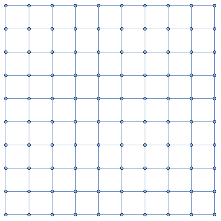
Out[]=
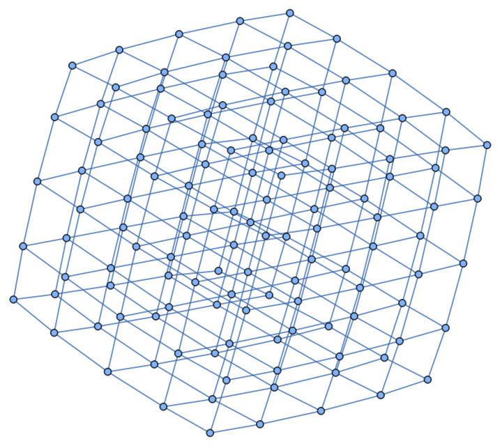
Recall that for a sphere in , the volume it encompasses is given by the formula , where r is the radius of the sphere and n is the dimension the space the sphere is in. Indeed, one can replicate a discrete version of the sphere volume formula using lattices. If x∈L, where L ≃, then I have let (x) to be defined as
n-1
S
n
n/2
π
(n-1)!
n
r
n
V
r
V
r
where d(x,y) denotes the shortest distance between two vertices in a graph. In the 2D plane, the points of ((0,0)) with r∈{0,...,4}
V
r
I highlighted the elements of the ball that have distance less than or equal to 0, 1, 2, 3, and 4 respectively. I used NeighborhoodGraph to find those elements that suffice that distance.
V
r
In[]:=
g=GridGraph[{9,9}];GraphicsRowTableHighlightGraphg,{NeighborhoodGraph[g,41,r]},,{r,0,4}
Out[]=
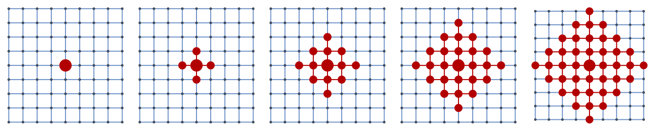
indeed, one can determine that the number of elements of can be represented as the polynomial 1+2r+2. I also considered the sub-lattice growing in (here, I have r∈{0,...,5}),
V
r
2
r
3
Simply the three-dimensional case of the integral grid:
In[]:=
t=GridGraph[{7,7,7}];GraphicsRowTableHighlightGrapht,{NeighborhoodGraph[t,172,r]},,{r,0,4}
Out[]=

here, the polynomial that represents the number of elements is +2++1. Indeed, one can generalize this into d-dimensions using the methods proposed by John B. Conway and Neil J. A. Sloane originally used to find the coordinate sequences for the root systems of associated Lie algebras. Let us define the following subsets of L⊂
4
3
r
3
2
r
8r
3
n
=
V
r
<
V
r
Clearly, I have that =⋃. Now, let us consider a new type of polytope called the contact polytope of a lattice L. This is defined to be the convex hull of the shortest lattice points (points with the least distance from the origin) and will always be denoted by C. We define the fractional height a point in a lattice x∈C to be
V
r
<
V
r
=
V
r
fht(x)={x∈hC}
min
h⩾0
where hL is simply L but each of the points are scaled by h in . Thus, we also have synonymous definitions of using fractional height. Each of the synonymous definitions can be defined as follows:
n
V
r
V
r
'<
V
r
'=
V
r
Where |*| denotes cardinality in this case.
Proposition 1.1.1 (Conway & Sloane):
A point x∈L has fractional height h iff it can be written in the form
Proposition 1.1.1 (Conway & Sloane):
A point x∈L has fractional height h iff it can be written in the form
x=,
d
∑
i=0
c
i
v
i
with the rational and nonnegative, Σ=h, and ,..., are the distinct minimal vectors of L that belong to a face of the contact polytope.
c
i
c
i
v
1
v
d
Consider the points of distance n from the origin in the cubical lattice. One can, by Proposition 1.1, represent these points as a linear combination as the minimal vectors of L with nonnegative coefficients that sum to n. Thus, if one were to consider all possible real coefficients that sum up to n, then one would obtain all of the elements of nC. Therefore, one can derive this theorem.
Theorem 1.1.1 (Conway & Sloane):
The points of fractional height at most h are all the lattice points in or on hC. The points of height at most n∈ are a subset of the lattice points within nC. Additionally, if we have that fht(x)⩽ht(x) for all x∈L, ⊃ for all n∈, and that ⌈fht(x)⌉⩽ht(x) iff =.
c
i
Theorem 1.1.1 (Conway & Sloane):
The points of fractional height at most h are all the lattice points in or on hC. The points of height at most n∈
>0
V
r
V
r
>0
V
r
V
r
The condition that fht(x) =⌈fht(x)⌉ for a lattice L makes L a well-placed lattice. Conversely, ⌈fht(x)⌉=ht(x) makes L well-rounded. Indeed, as an application of Ehrhart’s reciprocity theorem, we can express the number of elements in and as a polynomial that uses r as the independent variable.
Theorem 1.1.2:
For integral nonnegative r, and are respectively given by polynomials and in r of degree d, satisfying
V
r
'<
V
r
Theorem 1.1.2:
For integral nonnegative r,
V
r
'<
V
r
v
r
'<
v
r
v
-r
d
(-1)
'<
v
r
Furthermore, =1 while, for r>0, is the polynomial of degree d-1 satisfying =1-.
'=
V
0
'=
V
r
'=
v
r
'=
v
0
d
(-1)
I can now use these results to find the general formula for . Notice that for integral r>0, =- by definition. For a well-rounded lattice L, we can represent as a polynomial of r of degree d-1. This is due to the fact that we have that = by Theorem 1.1. To actually find , one can use the following arithmetic generating function
v
r
=
V
r
V
r
V
r-1
V
r
v
r
V
r
V
r
=
V
r
=
V
∞
Σ
r=0
=
V
r
n
x
So, since is of degree d-1, one can express it as +...+r+ for some constants . However, for the sake of simplicity, I will not use the standard polynomial form of this polynomial but instead express it in terms of , . Indeed, it is a fact that every polynomial of x of finite degree can be expressed as the linear combination of the binomial coefficients . Therefore, there exists constants such that =
. So,
=
V
r
a
d-1
d-1
r
a
1
a
0
a
i
r |
d-1 |
,...,
r |
d-2 |
r |
0 |
x |
i |
b
j
=
V
r
d-1
∑
n=0
b
n
r |
d-1 |
=
V
∞
Σ
r=0
d-1
∑
i=0
b
n
r |
i |
r
x
b
d-1
∞
Σ
r=0
r |
d-1 |
r
x
b
d-2
∞
∑
r=0
r |
d-2 |
r
x
b
0
∞
∑
r=0
r
x
Take a term of this sum, say,
. Notice that
=, and so the term must be equal to . Therefore, we have that (x) is equal to:
b
i
∞
∑
r=0
r |
i |
r
x
∞
∑
r=0
r |
i |
r
x
i-1
x
1-
i
x
b
i
i-1
x
i
(1-x)
=
V
b
d-1
d-1
x
d
(1-x)
b
d-2
d-2
x
d-1
(1-x)
b
0
1-x
b
d-1
d-1
x
b
d-2
d-2
x
d-1
b
0
d
(1-x)
P
d
d
(1-x)
where (x) is a polynomial of degree d-1. Now, I will consider the arithmetic generating function . Recall that =- as I have already mentioned. Therefore, one would obtain the following.
P
d
V(x)=
∞
∑
r=0
V
r
r
x
=
V
r
V
r
V
r-1
=
V
∞
Σ
r=0
=
V
r
r
x
∞
Σ
r>0
=
V
r
r
x
∞
∑
r>0
V
r
r
x
∞
∑
r>0
V
r-1
r
x
∞
∑
r=0
V
r
r
x
∞
∑
r=0
V
r
r
x
=1+(V(x)-1)-(xV(x))=V(x)-xV(x)
So,
=
V
=
V
1-x
Therefore, I have obtained the following theorem.Theorem 1.1.3:Let L be a well-rounded lattice. Then, I have that =(x), where (x) is a d-1 degree polynomial and that (x)=V(x).
=
V
r
P
d
d
(1-x)
P
d
=
V
1-x
Now, I am ready to find the formula for in . We already have that is well-rounded since the points are integral. In fact, for any , . Recall that a coordination sequence of a lattice L is given by {,,...}. The coordination sequence of is clearly {1,2,2,...}, and so we must have (x)=. Since ≃...(dtimes), we must have in d dimensions (x)=. Notice that we can write =
by the binomial theorem and =
by an argument involving multiple differentiation. Therefore:
V
r
d
d
x=(,...,)∈
x
1
x
1
d
ht()=fht(x)=||
d
∑
i=1
x
i
=
V
0
=
V
1
=
V
1+x
1-x
d
=
V
d
(1+x)
d
(1-x)
d
(1+x)
∞
∑
n=0
d |
n |
n
x
-d
(1-x)
∞
∑
m=0
d+m-1 |
d-1 |
m
x
Honeycomb (and Hexagonal) Case
Honeycomb (and Hexagonal) Case
Same method as the previous graphics, albeit with ResourceFunction[“HexagonalGridGraph”]:
and so this is equal to
Same method as before, albeit with ResourceFunction[“TriangularGridGraph”]:
Quasi-polynomials
Quasi-polynomials
Definition 1.3.2:
A quasi-polynomial q defined on the integers can be written as
A quasi-polynomial q defined on the integers can be written as
Setup and Motivation
Setup and Motivation
For example, take our previous grids. Note that each lattice can be realized as a free abelian group of rank d, where d is the dimension of the space the lattice is imbedded in. Therefore, if we take the lattice L = G, then it must have that L freely acts on itself by coordinate addition and that G/L = 1, 1 being the neutral element.
Magnitude
Magnitude
Therefore, I can define the magnitude of a graph G to be
Notice that
Magnitude Homology
Magnitude Homology
While magnitude homology may seem contrived and somewhat unrelated to the actual magnitude factor, there is a theorem that relates the ranks of each of the homology groups to the magnitude of a graph G.
Finally, one must characterize disjoint unions of graphs to magnitude homology. Like any homology theory, direct sums of homology groups are isomorphic to the homology group of a disjoint union of topological spaces. Similar to those theories, magnitude homology also follows the same behavior.
is an isomorphism. ◼
Indeed this is exactly the disjoint union axiom of a homology theory.
So, one can obtain this rather interesting theorem.
◼
Future Directions
Future Directions
Persistent Homology and Hausdorff Dimension
Persistent Homology and Hausdorff Dimension
I then showcased the barcode of the persistent homology group.
One interesting application to persistent homology in this manner is determining the what the fractional dimension a space is. A paper by Benjamin Schweinhart titled Fractional Dimension and Persistent Homology of Random Geometric Complexes provided a result and method to calculate the fractional dimension (d-Alhfors regular measure) of any space. More specifically, he derived the following result using persistent homology
with high probability as n goes to infinity. ◼
Conclusion
Conclusion
Acknowledgements
Acknowledgements
I would like to thank my mentor Lusine Sukiasyan for her support and guidance throughout the project. I would also like to thank the TA’s for their support and fun times throughout this program. I would also like to thank Stephen Wolfram for this program and this project I was offered. I would also like to Dugen and Pavel for offering very nice insights to my project that I haven’t considered before. Finally, I would like to thank room 280 and Hendry Xu for giving me a great experience in this program.
References
References
◼
Conway, J. H., & Sloane, N. J. A. (1997). Low–dimensional lattices. VII. Coordination sequences. Proceedings of the Royal Society of London. Series A: Mathematical, Physical and Engineering Sciences, 453(1966), 2369–2389. https://doi.org/10.1098/rspa.1997.0126
◼
The Notion of Dimension: Wolfram Physics Project Technical Background. (2026). Wolframphysics.Org. https://www.wolframphysics.org/technical-introduction/limiting-behavior-and-emergent-geometry/the-notion-of-dimension/
◼
Schweinhart, B. (2020). Fractal dimension and the persistent homology of random geometric complexes. Advances in Mathematics, 372, 107291. https://doi.org/10.1016/j.aim.2020.107291
◼
Häusermann, Nadja. (2024). Magnitude Homology, https://people.math.ethz.ch/~skalisnik/theses/Haeusermann_Msc.pdf
◼
Hepworth, R., & Fullerton, S. (2017, December). Categorifying the magnitude of a graph - White Rose Research Online. Whiterose.Ac.Uk. https://eprints.whiterose.ac.uk/id/eprint/116307/
◼
Inoue, T., & Nakamura, Y. (2024). Ehrhart theory on periodic graphs. Algebraic Combinatorics, 7(4), 969–1010. https://doi.org/10.5802/alco.367
◼
LEINSTER, T. (2017). The magnitude of a graph. Mathematical Proceedings of the Cambridge Philosophical Society, 166(2), 247–264. https://doi.org/10.1017/s0305004117000810