We construct a 2D spin network which serves as a toy model for a time slice of a (2+1)d black hole. We use the length operator, analogous to the area operator in loop quantum gravity, to determine the Bekenstein-Hawking entropy of the spin network at a certain graph distance. We only allow the spin network to be labeled by q-deformed SU(2) representations so that the edges are constrained to a maximum angular momentum eigenvalue during it’s evolution. We find that the entropy of the black hole horizon increases along with number of possible relabelings (evolutions) as we allow edges to have higher spin representations. We also find the circumference per graph distance, averaged over every node in the spin network, increases linearly following the black hole perimeter law.
Introduction
Introduction
Spacetime in Loop Quantum Gravity
Spacetime in Loop Quantum Gravity
Loop quantum gravity is an attempt to find a plank scale model of spacetime by triangulating a spacelike hypersurface of the manifold and quantizing geometric variables such as the metric triad and the spin connection [2]. The quantum properties of hypersurface after triangulation are easily encoded in the dual graph, a spin network, which is trivalent in (2+1)d (see fig 1a.). The edge of the spin network that pierces a face of the triangle is labeled by an unitary irreducible representation of SU(2), with the dimension being determined by the value of the area of the face, or in (2+1)d- the side length. The vertex of the spin network is labeled by an SU(2) intertwiner, which in the case of 3D gravity is the Clebsch-Gordan coefficients or Winger 3-j symbol, and encodes the volume of the triangle it centers. These two interpretations can be visualized in fig 1b, where representation assigned to an edge quantifies the area of contact between the two regions of discretized space. The triangle equality must hold quantum mechanically, which motivates the spin network property that the value of any two edges connected to a vertex of the trivalent network must be greater or equal to the third edge. This is the same mathematics behind the addition of two particles with spin degrees of freedom, known as the Clebsch-Gordon condition, which is typically shown in an undergraduate quantum mechanics course. It now becomes obvious why vertices come with a intertwiner, (Winger 3-j symbol in (2+1)d), as a means of relating the representations of the three connected edges.
Out[]=
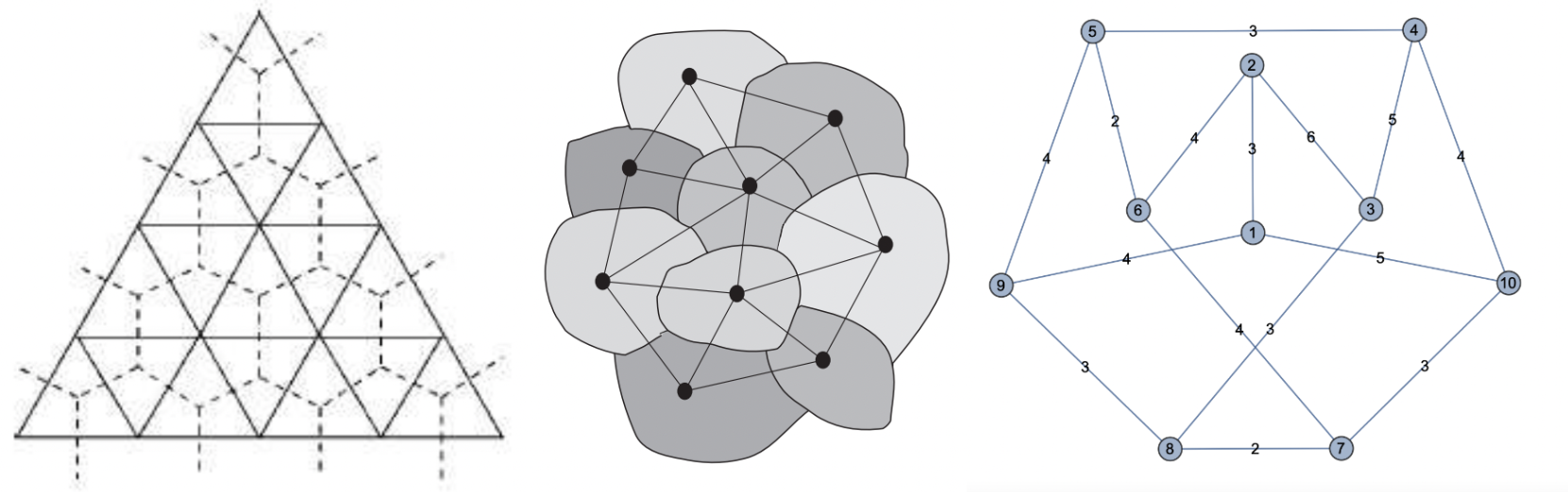
Fig 1. Fig[1a] (left), an example of a triangulation of a manifold (solid line) and it’s dual graph which is a trivalent spin network (dotted line). Fig[1b] (middle), a spin network and volumes of space associated to each vertex which the spin network models. Fig [1c](right), an example of a spin network properly labeled by the triangle inequality.
Black Hole Entropy in Loop Quantum Gravity
Black Hole Entropy in Loop Quantum Gravity
Since the 1970’s researchers have realized that black holes behave like a thermodynamic system with a twist; the entropy is determined by the area of the event horizon of the black hole and not it’s volume. This is commonly known as the Bekenstein-Hawking formula[3] and has been generalized to arbitrary dimensions[4]. Loop quantum gravity reproduces the Bekenstein-Hawking formula for macroscopic black holes by fixing the only free parameter in the theory, Barbero–Immirzi parameter. The choice of parameter remains the same for multiple black hole scenarios. A full quantum theory of black holes remain elusive in loop quantum gravity, so the conditions which we can consider a spin network a black hole are unknown.None the less, we will perform our analysis on arbitrary spin networks as if they are black holes in hopes of finding a relationship between the area of the horizon and the number of possible edge re-labelings (“microstates”) of a given spin network. The area of a given region in the spin network is determined by the area operator, having the spin networks are eigenstates, given by the formula: 8π(+1), where the i’s run over all the edges which puncture the 2D space that the area operator is defined on and is the representation of that edge. The area of an event horizon is then computed by applying the area operator to the edges which puncture a sphere representing that horizon [see fig 2a].
A
2
l
p
∑
i
j
i
j
i
j
i
Out[]=
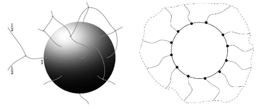
Fig 2. Fig[2a](left), an event horizon sphere penetrated by a spin network in (3+1)d. Fig[2b](right), a (2+1) event horizon circle being penetrated by a spin network.
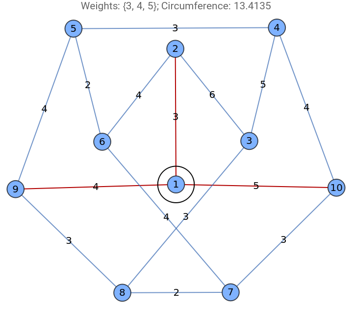
In (2+1) dimensions, the Bekenstein-Hawking entropy of a blackhole is then proportional to the circumference of the event horizon instead of the area [5]. In loop quantum gravity, the length operator takes the same form as the area operator: 8π(+1), i again running over the edges that pierces the circle (event horizon) on a spin network. Below you can interactively witness how the length of the horizon changes as different edges of the spin network are intersected (courtesy of Nikolay Murzin) .
L
2
l
p
∑
i
j
i
j
i
spinnet2=Graph[{1,2,3,4,5,6,7,8,9,10},{12,91,101,23,26,34,38,410,45,56,59,76,107,78,89},EdgeWeight->{123,914,1015,236,264,345,383,4104,453,562,594,764,1073,782,893},VertexCoordinates{},EdgeLabels"EdgeWeight",VertexLabelsPlaced[Automatic,Center],VertexSize0.2];embedding=AssociationThread[VertexList[spinnet2],GraphEmbedding[spinnet2]];weights=AssociationThread[EdgeList[spinnet2],AnnotationValue[spinnet2,EdgeWeight]];DynamicModule[{center=First@Nearest[Values@embedding,Mean@embedding],r=0.1,lines=Line@*List@@@Map[embedding,EdgeList[spinnet2],{2}],edges={}},Column[{Slider[Dynamic[r,(r=#;edges=Extract[EdgeList[spinnet2],Position[lines,l_/;!MatchQ[RegionIntersection[Circle[center,r],l],_EmptyRegion],{1},Heads->False]])&],{0,1}],Dynamic@Show[HighlightGraph[spinnet2,edges],Graphics[Circle[center,r]],PlotLabel->Row[{"Weights: ",Lookup[weights,edges],"; Circumference: ",Total@N@Sqrt[#(#+1)]&@Lookup[weights,edges]}],ImageSize->Medium]}],SaveDefinitionsTrue]
Out[]=
Method
Method
The interactive display is a bit naive since drawing the spin network in a different way can lead to different entropies. Also you can stretch the length of one of these edges. We want a precise, graph theoretic way to determine exactly which edges puncture a circle at a given radius. We will now give this procedure using the notion of graph distance as illustrated below. First we pick a vertex and find the vertices that are one edge or one graph distance away. Then we will find the set of vertices two graph distances away from the starting vertex. The edges which connect the vertices which are one graph distance away and two graph distance away from the starting vertex, we say pierces the event horizon when it is taken to be one “graph radius”. The circumference of the event horizon at cutting the spin network at two “graph radius” is determined by the representations on the edges which are connecting the vertices of two to three graph distance from the starting vertex, and so on. We define a “graph radius” of n as a circle intersecting the edges which link a vertex of graph distance n away to a vertex of a graph distance n+1 away.
Out[]=
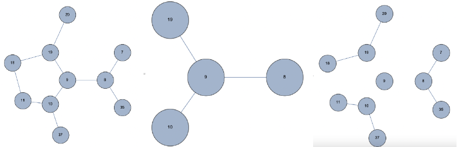
Fig 3. Fig[3 a] (left), contains all the vertices with a graph distance one and two away from the center vertex (9) . Fig[3 b] (middle) , contains all the vertices a graph distance one away from the center vertex (9) . Fig[3 c] (right), contains only the edges that connect vertices with a graph distance one and two away from the center vertex (9) . These are the edges that contribute to the first horizon at a "graph radius" of one .
Entropy per Graph Distance
Entropy per Graph Distance
In this section we will consider the entropy as a discrete function of graph distance. The term entropy is used interchangeably with the circumference of the “horizon” since the relationship between them in the full quantum theory is unknown. We show in the first subsection that only analyzing the entropy per graph radius around one vertex can yield bizarre answers and says little about black hole entropy as an intrinsic property of the graph. We find that if we average the entropy at a given graph radius over every vertex in the graph, the entropy is linearly proportional to the graph radius. This essentially reproduces the result the circumference of a circle is linearly proportional to it’s radius. Important Note: Every graph we will consider has a maximum spin representation of j=1/2 for every edge. In the next section, we argue why the geometric operators defined in the introduction are valid in this case, but in general they may not be when you restrict the dimension of possible representations.
Analyzing a Single Vertex is Not Sufficient
Analyzing a Single Vertex is Not Sufficient
We will start by analyzing the entropy per graph distance around certain points on the fullerene 80 vertex graph. We will see that for high values of graph distance the entropy starts decreasing, this is only due to the finiteness of the graph and is a feature of the graph distance reaching the graph’s boundary. In an infinite graph that would sufficiently model a meter-sized region of spacetime, since each side is of the order of a plank length, we do not expect any entropy decrease. If you expand the following subsections, you will find a plot of the entropy as a function of “graph radius” around a given vertex.
Out[]=
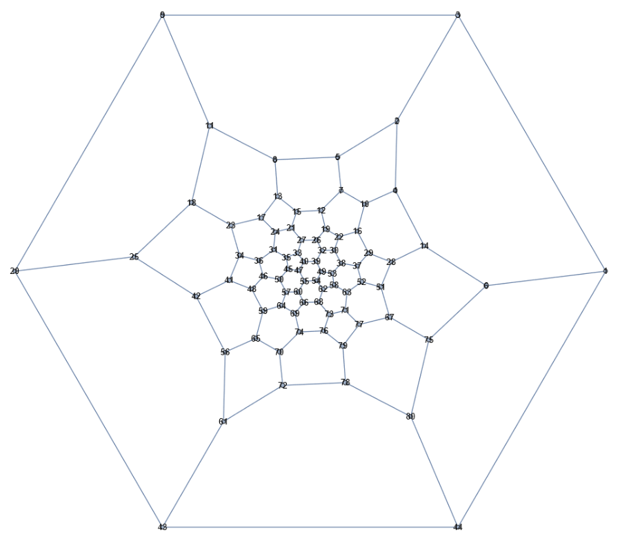
Entropy per Graph Distance around Vertex 47
Entropy per Graph Distance around Vertex 47
Entropy per Graph Distance around Vertex 9
Entropy per Graph Distance around Vertex 9
Average Entropy per Graph Radius for Various Graphs
Average Entropy per Graph Radius for Various Graphs
Here we will see that on average the entropy increases in an almost linear fashion. We will see that for high values of graph distance the entropy starts decreasing, this is only due to the finiteness of the graph and is a feature of the graph distance reaching the graph' s boundary. In an infinite graph, which would sufficiently model a meter - sized region of spacetime since each edge is of the order of a Plank length, we do not expect any entropy decrease .
Fullerene 80 Vertex
Fullerene 80 Vertex
Foster 200 Vertex
Foster 200 Vertex
Interlude on q -Deformed Algebras
Interlude on q -Deformed Algebras
Relationship between Black Hole Entropy and Number of Possible Spin Network Labelings
Relationship between Black Hole Entropy and Number of Possible Spin Network Labelings
In this section, we will find Bekenstein-Hawking entropy as well as the number of possible relabelings, as a discrete function of deformation variable r. Mathematica has difficulties finding these quantities in the method we used for even relatively simple graphs (such as 8 vertices) so we in this section we will consider one of the simplest trivalent graphs:
r = 3
r = 3
Plots
Plots
Conclusion and future goals
Conclusion and future goals
The results from section one match the geometric law in euclidean space that the circumference increases proportionally to the radius of the circle, in our case the radius is determined by the graph distance. For the particular relabellings we have considered, the graphs seemed to become more linear as we increased the vertex count up to 200. The main goal of this project was to explore the relationships between the number of possible relabelings of a graph and the circumference (black hole entropy) of the graph averaged over all the possible relabelings. We found that both the circumference and the possible relabelings of the graph increase as the deformation parameter increased, seeming to converge for large r. However, due to computational difficultly we were unable to consider r>22, so reaching conclusions about the relationship between circumference and number of possible relabelings for large r cannot be done at this time.
It might be possible to extend these calculations much farther if a combinatorial formula to compute the number of possible relabelings for a trivalent graph with a certain vertex number and deformation parameter is used. Also the graph considered in the last section is not the simplest trivalent graph, it should be interesting to see at what deformation parameter Mathematica can reasonably compute if we consider a two vertex trivalent graph.
It might be possible to extend these calculations much farther if a combinatorial formula to compute the number of possible relabelings for a trivalent graph with a certain vertex number and deformation parameter is used. Also the graph considered in the last section is not the simplest trivalent graph, it should be interesting to see at what deformation parameter Mathematica can reasonably compute if we consider a two vertex trivalent graph.
Keywords
Keywords
◼
Spin Network
◼
Loop Quantum Gravity
◼
Bekenstein-Hawking entropy
◼
BTZ black holes
◼
q-deformed algebra
Acknowledgment
Acknowledgment
I would like to thank my main leading mentor of this project, Mr. Alessandro Pisana, for giving me a much deeper understanding of loop quantum gravity in too many way to mention and always being there to answer any question I had in a swift and detailed fashion. I am in debt to Mr. Nikolay Murzin for supplying the basic code to begin all the computations, being there whenever I needed him, and patiently teaching me how to get much better at using Mathematica. I would like to thank Dr. Xerxes Arsiwalla for his meetings with me despite his busy schedule and being the first to suggest that I get a feel for black holes in loop quantum gravity. I also thank Dr. Stephen Wolfram for shaping the direction of this project and his insight into using a more graph theoretic approach. I would like to thank every one previously mentioned again as well as all the lectures for their perspective enhancing talks and the organizers for making the winter school a success.
I would like to thank Dr. Lorin Matthews and Dr. Gerald Cleaver for encouraging me to apply and to Dr. Anzhong Wang for our correspondence on loop black holes. I would like to thank Mr. Suvadeep Roy for being a supportive friend to discuss the winter school ideas with. I thank my family alot for supplying a warm, comfortable, and focused environment to complete the winter school.
I would like to thank Dr. Lorin Matthews and Dr. Gerald Cleaver for encouraging me to apply and to Dr. Anzhong Wang for our correspondence on loop black holes. I would like to thank Mr. Suvadeep Roy for being a supportive friend to discuss the winter school ideas with. I thank my family alot for supplying a warm, comfortable, and focused environment to complete the winter school.
References
References
◼
Mejrhit, K., R. Ahl Laamara, and S-E. Ennadifi. “On black hole radiation spectrum in loop quantum gravity.” Gravitation and Cosmology 23.1 (2017): 41-44.
◼
Rovelli, Carlo, and Francesca Vidotto. Covariant loop quantum gravity: an elementary introduction to quantum gravity and spinfoam theory. Cambridge University Press, 2015.
◼
Bekenstein, Jacob D. “Black holes and entropy.” JACOB BEKENSTEIN: The Conservative Revolutionary. 2020. 307-320.
◼
Wald, Robert M. “Black hole entropy is the Noether charge.” Physical Review D 48.8 (1993): R3427.
◼
Frodden, Ernesto, et al. “Statistical entropy of a BTZ black hole from loop quantum gravity.” Journal of High Energy Physics 2013.5 (2013): 1-17.
◼
Zachos, Cosmas. “Paradigms of quantum algebras.” Symmetries in Science V. Springer, Boston, MA, 1991. 593-609
◼
Dupuis, Maïté, and Florian Girelli. “Observables in loop quantum gravity with a cosmological constant.” Physical Review D 90.10 (2014): 104037.
◼
Chen, Jian-Zhen, and Jian-Yang Zhu. “Self-organized critical behavior: the evolution of frozen spin networks model in quantum gravity.” International Journal of Modern Physics A 23.24 (2008): 3891-3899.