The Wolfram Model is a class of models consisting of a graph (or hypergraph) and a rewriting rule. It has been shown by Wolfram [S. Wolfram, 2020] and Gorard [J. Gorard, 2021] that the Wolfram Model can exhibit behavior corresponding to general relativity in the continuum limit; however, it remains unknown precisely which rules show this correspondence. In this project, I conducted a systematic search over the space of possible rewriting rules to identify rules that preserve the geometric structure of graphs that correspond to static vacuum solutions of the Einstein equations, a necessary condition for these rules to satisfy general relativity. I considered rules involving 2 and 3 edges on simple directed graphs corresponding to flat Minkowski and Schwarzschild solutions. From a search space of 49,116 rules, I identified 32 rules that preserve geometric structure and may be candidates for modeling general relativistic behavior.
Introduction
Introduction
A foundational principle of the Wolfram Physics Project (WPP) is that spacetime is discretized at small scales and may be represented as a (hyper)graph structure that evolves according to the action of a hypergraph rewriting rule[1]. This concept is known as the Wolfram Model. This contrasts with the traditional view in General Relativity, where spacetime is represented as a continuous Riemannian manifold evolving according to a set of partial differential equations (the Einstein equations). The question then arises of how these views can be reconciled. It has been shown that a latent manifold structure can be recovered from certain hypergraphs in an appropriate continuum limit[1][2], and that certain classes of rewriting rules result in hypergraph evolution that satisfies the Einstein equations. However, not all rewriting rules will produce hypergraphs with a manifold structure. It remains an open problem in the Wolfram Physics Project to understand which rules give rise to manifold structure and satisfy the Einstein equations in the appropriate limit.
Consider a manifold that corresponds to a static solution of the Einstein equations. One necessary (but not sufficient) property for a suitable rewriting rule is that its action on a hypergraph with such a manifold structure should preserve the overall manifold structure upon repeated application. In this project, we conduct a systematic search for rewriting rules that preserve static manifold structure for flat Minkowski spacetime as well as for the Schwarzschild solution.
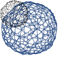
In a Wolfram Model, the hypergraph is typically constructed starting with a minimal initial condition, such as a single node with several self-loops. For this project, I will instead prepare an initial hypergraph that is constructed to have a latent manifold structure corresponding to the static solution of interest. These initial conditions may be considered a model of a “patch” (connected sub-graph) taken from a larger hypergraph that may have been produced through rewriting. Since we are only considering static solutions, we can simplify the problem by taking a hypergraph corresponding to a spacelike hypersurface and considering its evolution under the rule rather than considering the full causal graph (the analog of spacetime in the Wolfram Model).
In this project, I will first consider the role of the graph “microstructure” and establish criteria to bound the search space of rules. Specifically, we will look at rules involving 2 and 3 edges on simple directed graphs. I will then define heuristics to test rules for physical behavior. Subsequently, I will conduct an exhaustive search over the space of rules, applying the rules to four example initial graphs corresponding to flat space in two dimensions and evaluating the heuristics for each rule. Rules that pass the heuristic tests are then applied to a larger input graph corresponding to a Schwarzschild solution and re-evaluated. Additional tests are performed on the rules to check for triviality (isomorphism) and preservation of the graph’s Wolfram-Hausdorff dimension[1]. From these tests, 32 rules are identified from the initial search space of 49,116 rules.
Microstructure and Macrostructure
Microstructure and Macrostructure
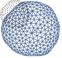
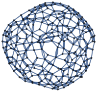
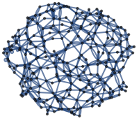
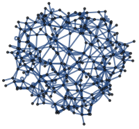
We have discussed that the macrostructure of the hypergraph may correspond to a latent manifold structure, however there are many possible hypergraphs that have equivalent coarse-grained macrostructure. These graphs are differentiated in terms of their microstructure, i.e. the detailed graph structure at short range. For example consider the following graphs:
Out[]=
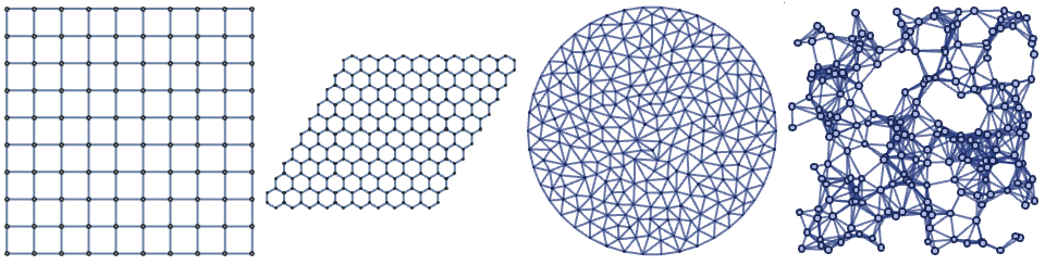
Each of these graphs have a macrostructure corresponding to two dimensional Euclidean space, however they differ in their microstructure. The first has a rectangular grid structure, the second is a hexagonal grid, the third is a triangular mesh and the fourth is produced by connecting a set of random vertices (“random sprinkling”).
Hypergraphs generated from rewriting rules from a minimal initial condition often show emergent microstructure[1 Ch 4.1]. For example the rule:
Hypergraphs generated from rewriting rules from a minimal initial condition often show emergent microstructure[1 Ch 4.1]. For example the rule:
In[]:=
{{x, x, y}, {x, z, u}} -> {{u, u, z}, {y, v, z}, {y, v, z}}
Out[]=
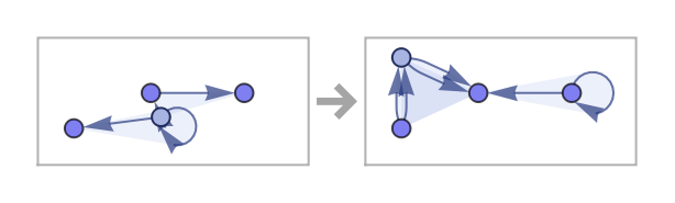
Produces the following hypergraph after 1000 steps:
Out[]=
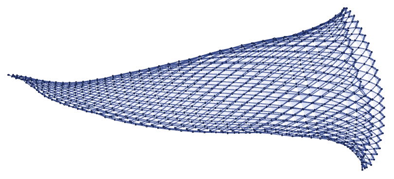
Where a clear repeated microstructure has become apparent.
It is possible that a rule may be manifold-preserving given one particular microstructure but not for another. As we am preparing model initial conditions that were not generated via rewriting, it is possible that the arbitrary choice of microstructure may impact our conclusions about the suitability of a rule. In this project I will also examine how the choice of microstructure impacts the behaviour of various rules.
The other major way in which our model differs from a hypergraph produced through rewriting is at the boundary. It is possible that the action of the rules at the boundary will differ from the behaviour of the sub-graph within a larger graph.
Enumerating the Space of Rules
Enumerating the Space of Rules
There are infinitely many possible rewriting rules. To perform a systematic search, we must constrain the search space. In this project I will apply the following constraints:
◼
All of our methods for preparing initial condition hypergraphs will generate simple directed graphs. Therefore there is no need to include rules involving hyperedges of more than 2 vertices, i.e. we can restrict our search to binary rules with signature[1 Ch 3.1] of the form .
N
2
M
2
◼
Rules which introduce new vertices or edges will quickly lead to exponential growth. Therefore we can further restrict our search to rules with the signature .
N
2
N
2
◼
It has been hypothesised that increasing the complexity of the rule (i.e. higher values of N) will not increase the complexity of the behaviour above some low threshold[1 Ch 3.11]. Previous results have shown does not show significantly more complex behaviour than , so we will not consider N>4.
2
2
5
2
2
2
4
2
There are 562 rules with signature , and 48,554 rules with signature . Using the formula from [1 Ch 3.2] for an estimate of the number of rules using Bell’s number, we can estimate the number of rules with signature is of order . As this is too large of a space to search systematically we will limit ourselves in this project to rules with the signatures and .
2
2
2
2
3
2
3
2
4
2
4
2
7
10
2
2
2
2
3
2
3
2
Criteria for Rule Selection
Criteria for Rule Selection
Testing the resultant hypergraph after rule application to determine if the manifold macrostructure has been preserved is a non-trivial task. There are techniques to calculate the curvature of a hypergraph[1][2] but they can be computationally expensive and may require large graphs to converge sufficiently to the continuum limit. It is also expected that a large fraction of possible rules will result in more obvious pathologies. To provide a fast and computationally efficient way to down select the set of rules we can use a set of heuristic tests to determine if a rule exhibits non-physical behaviour after only a few rounds (“generations”) of rule application.
The rule should:
The rule should:
1
.Not result in disconnected sub-graphs
2
.Not cause the number of vertices and/or edges to grow exponentially
◼
Note: it is possible to imagine a scheme where the graph “subdivides” while preserving macroscopic structure but this would not be compatible with the way typical Wolfram Models equate graph distances with metric distances and would require a more complex metric on the hypergraph to preserve lengths and volumes over time. I will exclude this possibility for now.
3
.Result in non-zero number of updating events
◼
Note: it is possible that a suitable rule would behave such that it results in no updating events in “empty” space but does behave correctly in the presence of “particles” or other dynamical structures. As in this project we only model static vacuum solutions, it is not possible to further evaluate these rules for suitability.
4
.Preserve approximate dimensionality
◼
We will measure this by computing the graph diameter and constraining the graph diameter not to shrink below a threshold compared to its initial value. As the number of vertices is approximately constant this crudely approximates that dimensionality is preserved.
For this project I will use a threshold for graph diameter of 50% of the initial value and a threshold for vertex and edge growth of 20% compared to the previous generation.
Evolution of an Example Graph
Evolution of an Example Graph
We begin by examining a few concrete examples of rule behaviour when applied to the mesh graph:
Out[]=
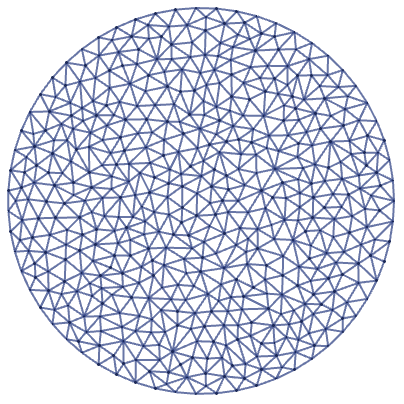
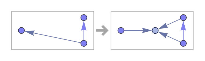
Starting with the rule {x,y},{x,z}}{{x,z},{y,z}:
In[]:=
(ruleEx2={{x,y},{x,z}}{{x,z},{y,z}}//ResourceFunction["CanonicalWolframModelRule"])//ResourceFunction["WolframModel"]//RulePlot
Out[]=

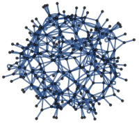
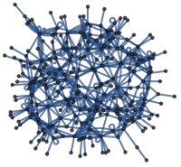
we can tabulate the evolution of the graph for each generation. For each generation I compute a variety of measures on the graph and check for the above criteria. If the graph fails one of the criteria we terminate the evolution. For this rule, the graph passes all tests for the first 5 generations:
Out[]=


For the rule {{x,y},{x,z}}{{x,z},{x,w},{y,w},{z,w}}:
Out[]=
We see that after one generation the rule fails the Δvertex and Δedge tests as shown in the column “Termination Criteria”. This is expected as the rule introduces a new vertex on each event and therefore will grow exponentially.
In[]:=
RunExperiment[None,graphToWolframModel[graphMesh2D],ruleEx1,5]
Out[]=
For the rule {{x,x},{x,x}}{{x,x},{x,x}}:
Out[]=
as our input graph does not contain self-loops this rule will not be applied and there will be no events:
Examples of Graph Evolution
Examples of Graph Evolution
In this figure we can see a variety of behaviour. Some graph appears unchanged by the rule. These correspond to rules that transform the graph in some trivial way such as flipping the direction of the edges. Some rules resulted in disconnected subgraphs, these will not be carried forward to subsequent generations. Others result in a rich variety of resultant structure.
To see the impact of different choices of microstructure we can perform the same procedure on the hexagonal grid. This graph shares the same flat macrostructure but shows significantly different behaviour:
To see the impact of different choices of microstructure we can perform the same procedure on the hexagonal grid. This graph shares the same flat macrostructure but shows significantly different behaviour:
Systematic Search with Flat Two-Dimensional Graphs
Systematic Search with Flat Two-Dimensional Graphs
For the first example of the mesh graph we can compute the percentages of each failure criteria, per signature:
We can immediately observe some features of the distribution of passing rules. There percentage of passing rules is around 2-5% so neither common nor particularly rare. There are large portions of the rule space that do not produce any events, and these regions are correlated but not identical between microstructures. To see how much commonality there is we can plot the passing rules coloured by how many graphs passed:
And computing the percentage of rules that pass with 1, 2 or all 3 of the input graphs:
Schwarzschild Graph
Schwarzschild Graph
We would like to test the behaviour of the rules with graphs corresponding to the Schwarzschild solution. To properly capture the geometric structure of the Schwarzschild solution it is necessary to use a graph with more vertices than used previously (the flat graphs had around 200 vertices). This proves to be computationally challenging so to constrain the search space we will only use the rules that passed for at least three out of four input graphs in the previous section. This leaves us with 719 rules to search over.
First we filter the rules by those that passed four generations without failing any criteria:
First we filter the rules by those that passed four generations without failing any criteria:
We repeat the search over just the passing rules from before, using a Schwarzschild graph containing 500 vertices. Note that due to the limitations of the graph generation functions, this graph represents a two dimensional spatial slice of the Schwarzschild solution, not a full three dimensional solution.
Each of the passing rules are then applied to the Schwarzschild graph for 4 generations and the heuristic criteria are evaluated.
This is a sample of the various behaviors of the Schwarzschild graph under the rules:
Now we can again analyze the termination criteria:
We can see that the majority of rules continue to pass with the Schwarzschild graph, however there are about 15% that fail.
Excluding Trivial Rules via Isomorphism
Excluding Trivial Rules via Isomorphism
By visual inspection of the sample above we can see some resulting graphs that appear unchanged by application of the rule. We know from the number of events that the rules do in fact apply, however it is possible that they result in a “trivial” transformation, for example swapping the directions of all edges. We can test for this by checking if the resulting graph is isomorphic to the original input. These rules may display physical behaviour in more complex systems (e.g. in the presence of dynamics or “particles”), however for the purposes of this study we cannot evaluate them further. By excluding these rules we can determine if there are non-trivial rules that also satisfy our criteria of geometry preservation.
The following plot shows the rules that result in an isomorphic graph highlighted in cyan:
We can see that about 6% of rules with 3 edges and 33% of rules with 2 edges result in isomorphic graphs.
Dimension Change under Rules
Dimension Change under Rules
Excluding rules that failed on the Schwarzschild graph as well as the trivial rules, we are left with 551 rules remaining. One property that our rules should have is to preserve the approximate curvature and dimension of the manifold. As our input graphs is still only 500 vertices, curvature estimates are “noisy”, however we can look more carefully at the change in dimension.
Our original criteria included a crude threshold on graph diameter that together with the threshold on vertex count acts to exclude rules that cause large changes in dimension, however this is not a very sensitive test. With our smaller search space we can instead plot the Δ(r) function[1] to get a finer grained view into how the dimension of the graph is effected by the rules.
In this plot each blue line corresponds to the resulting graph from a different rule. Each line shows Δ(r) as a function of r, averaged over 5 starting vertices around the graph center. The red line shows Δ(r) for the initial input graph. Note that it has a plateau around 2 as expected as the Schwarzschild solution was prepared as a 2D slice due to limitations of the graph generation function (generalizing to 3D is a topic for future work).
The plot shows that the rules can be grouped into 2 different behaviours. One group has Δ(r) spiking up at small values of r before quickly trending to zero. This corresponds to graphs that have become densely connected corresponding to higher dimension. There is a second group of rules that follow more closely the original input graph behaviour. To discriminate between these two groups it is sufficient to threshold on graph diameter > 13, these rules are now highlighted in orange:
Applying this threshold we are left with just 32 rules.
Results
Results
To recap we first did an exhaustive search over rules involving 2 and 3 edges using four small input graphs corresponding to flat two dimensional space. The graphs were evolved according to each of the heuristic criteria for four generation and those rules that passed all criteria for at least three out of four graphs were selected. These rules were then tested again on a larger Schwarzschild graph and filtered according to the criteria. Additional criteria for isometry and dimension preservation were applied resulting in 32 remaining rules. The 32 remaining rules are shown here together with the corresponding final state of the Schwarzschild graph after four generations:
The numbers of remaining rules per signature were:
Conclusions
Conclusions
◼
Systematic search using heuristic criteria can be a powerful tool for exploring the space of rules in the Wolfram Model.
◼
Suitable rules that preserve geometry are relatively rare for the cases we considered, comprising just 0.07% of rules evaluated, but several candidate rules were found.
◼
Sensitivity to microstructure is a significant challenge for systematic rule searches as we do not know what the correct vacuum microstructure(s) will be in Wolfram Models that correspond to physical behavior.
Future Work
Future Work
This project attempted to provide the simplest possible version of a systematic rule search and there are many possible avenues for future work:
◼
Extensions to larger graphs and longer evolutions
◼
Testing the full three dimensional Schwarzschild solution
◼
Trying more complex vacuum solutions such as the Kerr metric that include shear
◼
Using more sophisticated heuristics such as curvature measures (e.g. Olivier-Ricci curvature)
◼
Testing if these rules produce the expected dynamics in non-static or non-vacuum scenarios
◼
It may be possible to reason about the sensitivity to microstructure by finding equivalencies between classes of rules and microstructures
Use the Rules in your Project
Use the Rules in your Project
If you’d like to experiment with the rules from this project they are available from the Wolfram Data Repository:
Acknowledgments
Acknowledgments
I would like to thank my mentors, Nik Murzin and Xerxes D. Arsiwalla, for their guidance and support. I also thank Gianmarco Morbelli and Jon Lederman for the valuable discussions that contributed to this project. I would also like to extend my special thanks to Stephen Wolfram for suggesting this project and to all of the Wolfram Summer School team for putting together this fantastic program.
References
References
1
.S. Wolfram (2020), “A Class of Models with the Potential to Represent Fundamental Physics,” https://www.wolframphysics.org/technical-introduction/.
2
.J. Gorard (2021), “Some Relativistic and Gravitational Properties of the Wolfram Model”, arXiv:2004.14810v2 [cs.DM]
Cite This Notebook
Cite This Notebook