The vapor–liquid equilibrium (VLE) and liquid–liquid equilibrium (LLE) of the methanol–cyclohexane system at 0.1 MPa were modeled using the NRTL activity coefficient model. The system exhibits strong non-ideal behavior due to the polarity difference between methanol and cyclohexane, leading to significant deviations from Raoult’s law and partial liquid immiscibility.
VLE calculations were performed using the modified Raoult’s law with Antoine vapor-pressure correlations, while LLE conditions were obtained by satisfying equality of component activities in the two liquid phases. Experimental LLE data used for validation were taken from the work of Hiroyuki Matsuda, Kenji Ochi, and Kazuo Kojima.
The NRTL binary interaction parameters were obtained from the correlation of experimental LLE data reported by Zadjia Atik and Wahiba Kerboub, and implemented without modification.
The model successfully reproduces both the VLE azeotropic behavior and the LLE miscibility gap, showing good agreement with experimental data over most of the temperature range studied. The upper critical solution temperature (UCST - indicated by the green point) is slightly overestimated.
NRTL Parameters tau12,tau21: dimensionless interaction parameters (=Δg12/RT,Δg21/RT) alpha: non-randomness parameter (typically 0.2–0.47)
nrtlGex[x1_,tau12_,tau21_,alpha_]:=Module[{x2,G12,G21},x2=1-x1;G12=Exp[-alpha*tau12];G21=Exp[-alpha*tau21];x1*x2*(tau21*G21/(x1+x2*G21)+tau12*G12/(x2+x1*G12))]gmixRT[x1_,tau12_,tau21_,alpha_]:=Module[{x2},x2=1-x1;x1*Log[x1]+x2*Log[x2]+nrtlGex[x1,tau12,tau21,alpha]](*Derivative(chemicalpotentialdifference)*)dgdx[x1_,tau12_,tau21_,alpha_]:=D[gmixRT[x,tau12,tau21,alpha],x]/.x->x1(*Spinodal:solved²G/dx²=0*)spinodalPoints[tau12_,tau21_,alpha_]:=Module[{d2g,sols},d2g=D[gmixRT[x,tau12,tau21,alpha],{x,2}];sols=x/.NSolve[{d2g==0,0<x<1},x,Reals];Sort[sols]](*CommonTangent:solvethe2×2system-Conditions:(1)dG/dx|_{xa}=(G(xb)-G(xa))/(xb-xa)(2)dG/dx|_{xb}=(G(xb)-G(xa))/(xb-xa)*)commonTangent[tau12_,tau21_,alpha_]:=Module[{ga,gb,slope,eq1,eq2,guess,sol,xa,xb,sp},(*Initialguessfromspinodalbracket*)sp=spinodalPoints[tau12,tau21,alpha];If[Length[sp]<2,Return[{None,None}](*fullymiscible*)];guess={sp[[1]]*0.5,sp[[-1]]+(1-sp[[-1]])*0.5};ga=gmixRT[xa,tau12,tau21,alpha];gb=gmixRT[xb,tau12,tau21,alpha];slope=(gb-ga)/(xb-xa);eq1=D[gmixRT[x,tau12,tau21,alpha],x]/.x->xa;eq2=D[gmixRT[x,tau12,tau21,alpha],x]/.x->xb;sol=FindRoot[{eq1-slope==0,eq2-slope==0},{{xa,guess[[1]]},{xb,guess[[2]]}},MaxIterations->200,PrecisionGoal->8,AccuracyGoal->8];{xa,xb}/.sol]
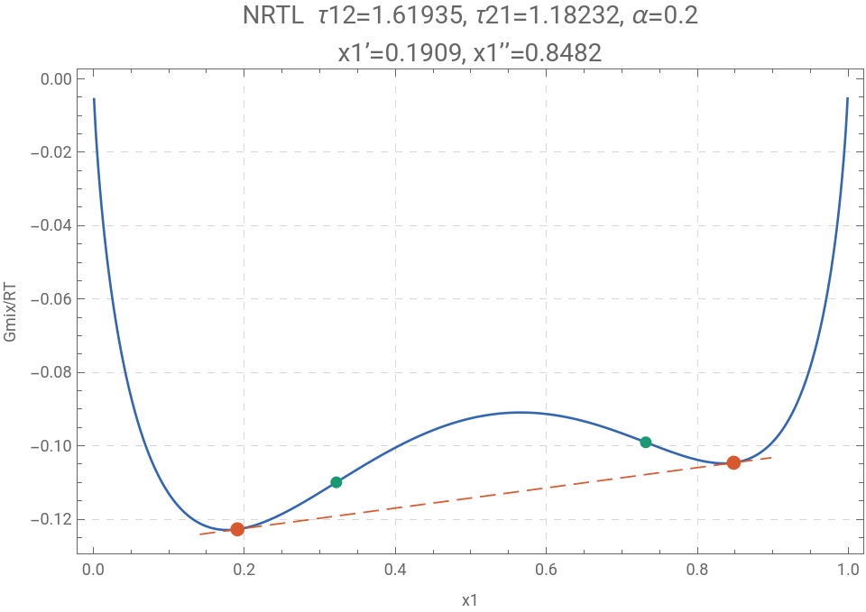
Single Gmix/RT curve with common tangent overlay
plotGmix[tau12_,tau21_,alpha_]:=Module[{xvals,gvals,ct,xa,xb,ga,gb,sl,tangentLine,curvePlot,tangentPlot,pointPlot,sp,spinPlot},xvals=Range[0.001,0.999,0.001];gvals=gmixRT[#,tau12,tau21,alpha]&/@xvals;sp=spinodalPoints[tau12,tau21,alpha];ct=Quiet@commonTangent[tau12,tau21,alpha];xa=ct[[1]];xb=ct[[2]];curvePlot=ListLinePlot[Transpose[{xvals,gvals}],PlotStyle->{RGBColor[0.2,0.4,0.7],Thickness[0.003]},PlotRange->All];If[xa=!=None,ga=gmixRT[xa,tau12,tau21,alpha];gb=gmixRT[xb,tau12,tau21,alpha];sl=(gb-ga)/(xb-xa);tangentLine={ga+sl*(#-xa),#}&/@{xa-0.05,xb+0.05};tangentPlot=ListLinePlot[Map[Reverse,tangentLine],(*swapto{x,y}*)PlotStyle->{RGBColor[0.85,0.35,0.18],Dashing[{0.02,0.01}],Thickness[0.002]}];pointPlot=ListPlot[{{xa,ga},{xb,gb}},PlotStyle->{RGBColor[0.85,0.35,0.18],PointSize[0.018]}];spinPlot=If[Length[sp]>=2,ListPlot[{{sp[[1]],gmixRT[sp[[1]],tau12,tau21,alpha]},{sp[[2]],gmixRT[sp[[2]],tau12,tau21,alpha]}},PlotStyle->{RGBColor[0.1,0.6,0.45],PointSize[0.015],PlotMarkers->{"▲",14}}],Graphics[]];Show[curvePlot,tangentPlot,pointPlot,spinPlot,Frame->True,FrameLabel->{"x1","Gmix/RT"},PlotLabel->Style[StringForm["NRTL τ12=`1`, τ21=`2`, α=`3`\nx1’=`4`, x1’’=`5`",tau12,tau21,alpha,NumberForm[xa,{4,4}],NumberForm[xb,{4,4}]],14],GridLines->Automatic,GridLinesStyle->Directive[GrayLevel[0.85],Dashed],ImageSize->480],(*Misciblecase*)Show[curvePlot,Frame->True,FrameLabel->{"x1","Gmix/RT"},PlotLabel->Style["NRTL — fully miscible",14],ImageSize->480]]]
Literature NRTL params from Ref. 1
Clear[T];tau12=2512.31/T-6.668;tau21=34.05/T+1.070;alpha=0.20;
In[]:=
T=303.15;
In[]:=
{tau12,tau21}
Out[]=
{1.61935,1.18232}
In[]:=
spinodalPoints[tau21,tau12,alpha]
Out[]=
{0.26823,0.678099}
In[]:=
commonTangent[tau21,tau12,alpha]
Out[]=
{0.151766,0.809059}
In[]:=
plotGmix[tau12,tau21,alpha]
Out[]=
In[]:=
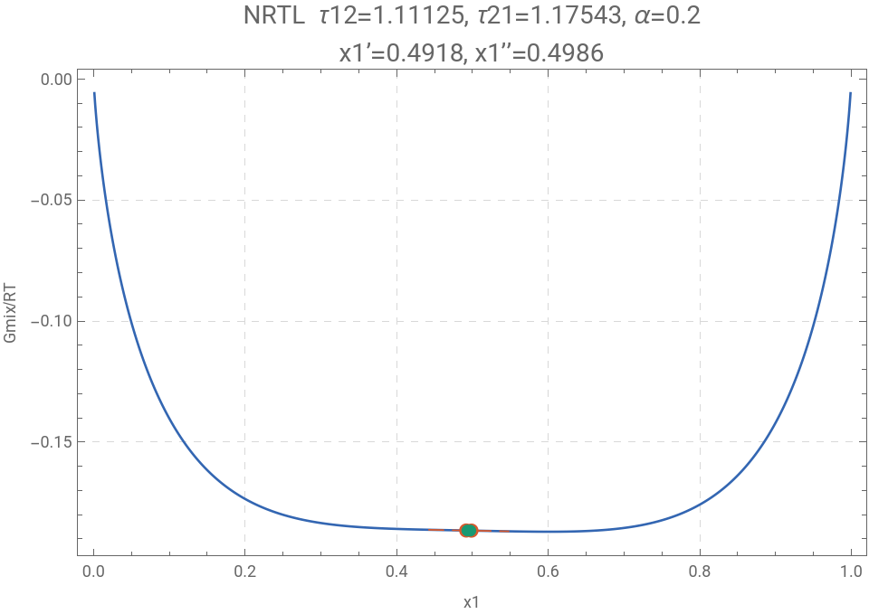
T=322.95;
In[]:=
{tau12,tau21}
Out[]=
{1.11125,1.17543}
In[]:=
spinodalPoints[tau21,tau12,alpha]
Out[]=
{0.502808,0.506743}
In[]:=
commonTangent[tau21,tau12,alpha]
Out[]=
{0.501368,0.508183}
In[]:=
plotGmix[tau12,tau21,alpha]
Out[]=
In[]:=
Clear[T]
In[]:=
LaunchKernels[]
Out[]=
KernelObject

In[]:=
mydata=Parallelize@Table[{i,Quiet@commonTangent[tau12/.T->i,tau21/.T->i,alpha][[1]],Quiet@commonTangent[tau12/.T->i,tau21/.T->i,alpha][[2]]},{i,273.15,323.0,0.01}];
In[]:=
mydatashort=Table[mydata[[i]],{i,1,Length@mydata,100}];
p1=Show[ListPlot[{Transpose@{mydatashort[[All,2]],mydatashort[[All,1]]-273.15},Transpose@{mydatashort[[All,3]],mydatashort[[All,1]]-273.15}},PlotMarkers->{Style["■",12,Darker@Gray],Style["■",12,Darker@Gray]},Frame->True,AspectRatio->1,GridLines->Automatic],ListPlot[{Transpose@{mydata[[All,2]],mydata[[All,1]]-273.15},Transpose@{mydata[[All,3]],mydata[[All,1]]-273.15}},PlotStyle->Darker@Red,Joined->True,Frame->True,AspectRatio->1,GridLines->Automatic],Graphics[{Darker@Green,PointSize[0.02],Point[{mydata[[-6]][[2]],mydata[[-6]][[1]]-273.15}]}],FrameLabel->{Style["Cyclohexane mole fraction",14],Style["T [°C]",14]},PlotRange->{{0,1},{0,52}}](*theuppercriticalsolutiontemperature(UCST)isindicatedbythegreenpoint*)
Activity coefficients using NRTL model
Component 1 = Cyclohexane
Component 2 = Methanol
Component 1 = Cyclohexane
Component 2 = Methanol
Vapor Pressure Using Antoine Equation
Gas Constant and Pressure
Computing VLE data
T-xy and xy plots for the 1Butanol-water system
References
References
[1] Matsuda, Hiroyuki and Ochi, Kenji and Kojima, Kazuo, Determination and Correlation of LLE and SLE Data for the Methanol + Cyclohexane, Aniline + Heptane, and Phenol + Hexane System, Journal of Chemical & Engineering Data, 48(1), pp. 184-189, 2003. DOI: 10.1021/je020156+
[2] Zadjia Atik and Wahiba Kerboub, Journal of Chemical & Engineering Data, 53(7), pp. 1669-1671, 2008 . DOI: 10.1021/je8001688
CITE THIS NOTEBOOK
CITE THIS NOTEBOOK
Binary LLE and VLE of methanol-cyclohexane mixture at 0.1 MPa
by Housam Binous
Wolfram Community, STAFF PICKS, June 7, 2026
https://community.wolfram.com/groups/-/m/t/3729140
by Housam Binous
Wolfram Community, STAFF PICKS, June 7, 2026
https://community.wolfram.com/groups/-/m/t/3729140