CITE THIS NOTEBOOK: Course models: Disease Ecology & Evolution, Evolutionary Medicine by Gareth Russell. Wolfram Community NOV 12 2022.
This notebook is the main resource for a module within the courses Disease Ecology and Evolution and Evolutionary Medicine at the New Jersey Institute of Technology.
Infectious Disease
Infectious Disease
An infectious disease is the population of a pathogen, distributed in space (host bodies). The distribution and dynamics of populations in space is part of the discipline of ecology. While some very simple disease models were developed a long time ago, they remained largely unchanged until the similarity between those models and new work in ecological modelling was noticed by a pair of mathematical ecologists: Roy Anderson and Robert May. In 1991 they wrote a book: Infectious Diseases of Humans: Dynamics and Control, and the field of epidemiology exploded from there. From a contemporary review:
This long and important book summarizes the results of nearly a decade and a half of collaboration between two of the world’s best analysts of infectious diseases and alludes to related work by many others… …The authors write, “The primary aim of this book is to show how simple mathematical models of the transmission of infectious agents within human communities can help to interpret observed epidemiological trends, to guide the collection of data towards further understanding, and to design programmes for the control of infection and disease. Our major goal is further understanding of the interplay between the variables that determine the course of infection within an individual, and the variables that control the pattern of infection.”
Models have two goals: understanding and prediction. They simplify reality on purpose. One important reason is tractability: complicated models can be too difficult to analyse and understand. Another reason is generality. The more complicated a model, the more likely it is to apply to a limited range of situations, or even just one, whereas we often want to understand a broad class of circumstances. Complexity is ok for something like a global climate model, because we are particularly concerned with one case — our own planet — and want to make accurate predictions about it. However an astronomer wondering about the ancient climate of Mars, and how it followed a different path from that of Earth, wants to understand planetary climates more generally. Infectious disease models are built on a simple, general base, which can then be customized and extended to add the details of specific diseases. Here we will be looking at that base.
Most infectious disease models simplify the world in the following two ways:
1
.They model the host, rather than the pathogen. A single infected human may host 100 billion viruses. The population of viruses within the host does have its own dynamics, which can be modeled, and because the pathogen population will correlate to some degree with adverse symptoms, these dynamics are of interest to clinicians tasked with caring for patients. But this is too much detail from the perspective of public health, which is concerned with the global spread of a pathogen. What matters there is whether a patient (host) is transmitting the disease to others, and this can be treated as a property of the host.
2
.They don’t even model individual hosts. In a large population it becomes difficult to model individual hosts (let alone pathogens), but luckily, large populations exhibit predictable average behavior. This is similar to the way that physicists can model most gasses using ‘mass action’ concepts like pressure and temperature, rather than worrying about the velocity and collisions of individual atoms and molecules. Of course sometimes it is necessary to model those things — generally when the number of elements being modeled is small — and at the end of this notebook are a couple of simulation models that do just that. But we will start with the basics.
So, all the models in this section are compartment models, meaning that they divide the population of hosts into different categories (‘compartments’), and model the number, or more commonly the fraction, of the host population in each compartment. The compartments can be any set of categories that are relevant to disease transmission, but we will start with the very simplest: a pair known as susceptible and infected…
The SI (Susceptible–Infected) model
The SI (Susceptible–Infected) model
In the SI model, individuals are either infected by a disease, or not infected and therefore susceptible to being infected. No-one is naturally resistant, and there is no recovery; infected individuals are infected for the remainder of their lives.

So this model is for a disease that is incurable, but doesn’t kill its host. In the past, there were many like this: think of the various STDs like chlamydia, gonorrhea, etc. A lot of these diseases are curable now, and so this model applies in only a few limited circumstances. We focus on it first because it is the simplest.
The key to the model is to recognize that, because an infection requires that an infected individual meets an uninfected (susceptible) individual, then the overall rate of infection of new individuals is given by the product of the number of susceptible () and the number of infected () individuals. This rate is typically represented by (meaning β × I × S) where is a constant that describes how likely it is that an infected individual infects a susceptible individual (it is usually called the transmission rate term). Thus we have two equations that describe rates of change, one for each compartment in the population.
S
I
βIS
β
dS
dt
dI
dt
These models of rates of change are differential equations. This is important: they describe the arrow in the diagram above (the rate of transition of individuals from one category to the other), not the compartments themselves (the number of individuals in each category). They are also symmetrical: one is just the negative of the other. If you think about it, that must be the case. There is only one arrow in the diagram; the two equations describe it from the perspective of the two compartments. Individuals leave the S compartment, so the rate is negative (the number in the S compartment will get smaller as a result). The same individuals enter the I compartment, so it’s the same rate, but positive.
Because no individuals are entering or leaving the system as a whole (just changing compartments), the total number of individuals will remain constant, which allows us to simplify how we describe the model. If we call that fixed total population size , where , we can also say that or . In other words, if we know N, which is fixed and doesn’t change, then if we also know the number of infected individuals, we automatically know the number of susceptibles (and vice versa). We therefore only need to model the dynamics of one of the compartments. Let’s say we do it for the infected group. We take the original equation and substitute :
N
N=S+I
S=N-I
I=N-S
S=N-I
dI
dt
Now we have a single equation, in a single variable (I), that models the dynamics of the whole system (because we can always get S from ). It is a simple form of the logistic equation, which you may have encountered in an ecology class.
N-I
What will happen in the long run? To answer that, we don’t need to do calculus; we can solve for zero (the condition, or fixed point, at which , meaning that the number of infected individuals remains constant).
dI/dt=0
0=βI(N-I)
This is just algebra! If you look at this equation, you should immediately see that there are at least three ways it can be true: if , if , or if (because then ). Let’s consider the meaning of these in turn. β is a constant representing the disease’s transmission rate, and if it can’t transmit, it’s not even an infectious disease at all, so this solution is called trivial, meaning that it’s true, but not useful or interesting. By definition, we are modelling something for which . The second solution, , is also somewhat obvious. If no-one is infected, then there can be no transmission, and as long as the population is closed (no immigration of possibly infected individuals), it will remain the case that no-one is infected. The third solution, , is also obvious. In this model there is no recovery, and so once everyone has been infected, there will be no more transmission.
β=0
I=0
I=N
N-I=0
β>0
I=0
I=N
Are these the only fixed point solutions? Is there a possible solution in which some fraction of the population is infected and that fraction remains constant? To work that out, let’s go back to the equation for the dynamics of the infected group:
dI
dt
Let’s consider the case when I is small, but not zero. As is the whole population, will be quite close to , and in any case will be a positive number. We know that beta is a positive number, and now we know that it is multiplied by a small positive number () and a larger positive number (). So overall, the right hand side of the equation is positive, which means the size of the group is getting bigger over time. What this tells us is that, once a disease like this enters a population (at low frequency), it will spread. Now consider the the case when is large (but not as large as ). Now is a large positive number , and is small positive number. (A sort of mirror image of the case when is small) But the important point is that again, both are positive, so is still increasing. By induction, we conclude that for any value of greater than zero but less than , will increase, which means that once an infection enters the population it will always increase until everyone is infected. We say that the the solution is absorbing.
N
N-I
N
I
N-I
I
I
N
I
N-I
I
I
I
N
I
I=N
This is a good time to also talk about stability. A long term fixed point is deemed a stable equilibrium if a small perturbation (deviation) from that point tends to return to it, and unstable if a perturbation tends to get bigger. By this definition, the solution is a stable equilibrium because if the value of is a bit less that this, we have shown that it will grow, i.e., return towards . Conversely, the solution is unstable, because if the value of is a bit more than zero, it will continue to grow, i.e., move further away from zero.
I=N
I
I=N
I=0
I
Finally, let’s consider the way in which the size of the group changes. It is useful to make a plot of the rate of change of I, , as a function of . We know from the equation above that =βI(N-I). Let’s assume that and .
I
dI
dt
I
dI
dt
β=0.01
N=100
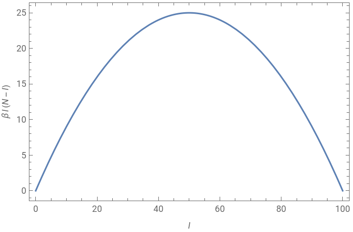
This shows graphically some of the things we already deduced: the growth rate is zero when and , and positive at all values in between. But it shows something else: the growth rate is maximum when . In other words, the most transmission occurs when half the population is infected and half is uninfected. This makes sense, as this is the state in which infected and uninfected individuals will be most likely to encounter each other.
I=0
I=N
I=N/2
Finally, what about the dynamics over time? To find that, we do have to do calculus (or have the computer do it!). We solve the differential equation for (time), which means integrating it. For a simple equation like this it can be done symbolically:
t
I(t)=
I(0)N
βNt
I(0)(-1)+N
βNt
where is the starting size of the Infected category. For those who are interested, here is the computer doing it:
I(0)
In[]:=
soln=FullSimplify[DSolve[{i'[t]β*i[t]*(n-i[t]),i[0]i0},i[t],t][[1,1]]]
Out[]=
i[t]i0n
ntβ
(-1+)i0+n
ntβ
Here what happens to over time, starting with an initial infection of 5 individuals.
I
Out[]=
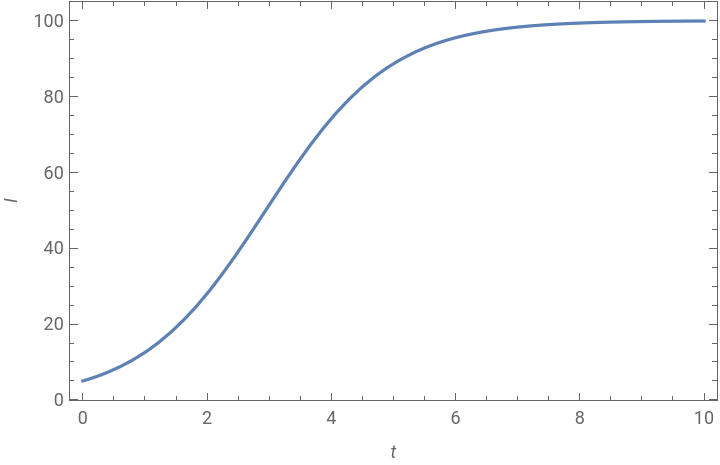
You will see that the maximum rate of increase in (the maximum positive slope) occurs at , i.e., , as predicted by the previous plot.
I
I=50
K/2
Now we will apply the same kind of reasoning to some (slightly) more sophisticated models!
The SIS (Susceptible–Infected–Susceptible) model
The SIS (Susceptible–Infected–Susceptible) model
The next simplest model — one that does describe many diseases — is one in which infected individuals recover with some rate (gamma) This is the susceptible–infected–susceptible, or SIS model.
γ

We still have a closed population of size N, and no (or at least negligible) disease-related mortality. So this applies to something like the common cold, or the milder childhood diseases such as measles. (There are no diseases with zero impact on mortality, but models simplify when it is reasonable to do so.)
The equations are now.
dS
dt
dI
dt
Can you see why? Think about how each compartment has two arrows connected to it, and which way they are going. Focusing on the infected population as before, and simplifying to one equation by substituting for :
N-I
S
dI
dt
Again, we ask: what are the long-term fixed points? Remember that this means solving the following equation:
0=βI(N-I)-γI
You should see that one of the answers from the SI model, , still applies. What about ? In that case, the first term on the right hand side, , will be zero, but the second term will be . As γ itself is positive, this whole term will be negative, so the whole of the right hand side becomes , which is negative, so the number of infected is decreasing. Put simply, some people are always recovering, and so the whole population can never stay infected. is not a fixed point.
I=0
I=N
βI(N-I)
-γN
0-γN
I=N
Because the righthand side of the equation now has two terms, one positive and one negative, you should be able to see that another way for it to come out to zero is for both these terms to have equal magnitude, and thus cancel each other out. This is when the infection rate equals the recovery rate. Mathematically we say that
0=βI(N-I)-γI
if
βI(N-I)=γI
Again, this is true if , but if we divide both sides by , you will see that it is also true if
I=0
I
β(N-I)=γ
We can rearrange this using the following steps to determine the fixed point for I.
N-I=
γ
β
-I=-N
γ
β
I=N-
γ
β
What does this mean? If is less than , then the fixed point of is a positive number: a number of infected individuals that will remain constant, because the rate at which new infections occur is the same as the rate at which infected individuals recover. But if is equal to or greater than , then the fixed point is (mathematically) zero or negative, and as we can’t have negative numbers of people in the real world, what that means is that the number of infected will decline to zero: the disease will die out.
γ/β
N
I
γ/β
N
Next we should consider the stability of this fixed point: the one where . It’s easier to do this graphically. See your class notes!
β(N-I)=γ
Before we move on to other models, we need to talk about a trick mathematicians use to make their lives a bit easier. Until now, we have had a constant in our models: the total population size. Mathematicians don’t like constants: they would like as few of them as possible. And we can, in fact, get rid of if we simply assume that and , instead of being numbers of actual individuals, are instead fractions of the total population N. In that case must add up to 1 (instead of ), and we can rewrite our equations with 1 where we had before. For example:
N
N
S
I
S+I
N
N
dI
dt
The solution to this is now
I=1-
γ
β
This result would look familiar to an ecologist; it’s the Levins metapopulation model! ( is equivalent to and is equivalent to .) The systems are entirely analogous — a disease is a population divided into patches, where the patches are individuals, and disease transmission and recovery is equivalent to colonization and extinction of patches.
e
γ
c
β
Reproductive rate R, and R0
Reproductive rate R, and
R
0
If you have ever watched a documentary, or even a Hollywood movie, about disease, you will likely have heard a reference to (“R-zero”), the most important number in epidemiology,
R
0
Epidemiologists define the reproductive rate of the disease as the incoming rate to the infected category (rate of new infections) divided by the outgoing rate (in this case, this is the rate of recovery). So for the ‘fractions’ version of the SIS model:
R
R==
βIS
γI
βS
γ
This number varies over time as I and S, the fractions of infected and susceptibles, change. So we define the basic reproductive rate, of the disease as the reproductive rate when a single individual is introduced into a large population of susceptibles, in other words, as (and therefore , which is where the 0 in comes from).
R
0
S1
I0
R
0
R
0
β
γ
This no longer depends on , and so is a constant. If >1, meaning that , then the rate of infections caused by an individual are greater than that individual’s recovery rate. It is the threshold for an epidemic. For smallpox, ≈4; for rubella, ≈8; for measles, ≈20 — all well above 1.
S
R
0
β>γ
R
0
R
0
R
0
What happens to R over time? It depends on the model. For the SI model as presented above, R and can’t be defined , because there is no recovery, so we are dividing by zero. Or to put it another way, mathematically, . But that is an artifact of the model being so simplified. The denominator is meant to capture the period of time in which people are contagious. They may not recover, but people don’t live forever either, so the lowest possible rate is not really zero, it is the inverse of the average lifespan of a person. Which is still a small number, so R and are still going to be relatively large, but that’s not surprising because if you don’t recover from a disease, and remain contagious for the remainder of your entire life, you are likely to infect a lot of people!
R
0
R=∞
R
0
For the SIS model, with recovery, we can make a graph of R over time. First, this is how I, the total number of infected people, changes over time from a very small number. It grows to the steady state, which we saw above is given by .
I=N-
γ
β
Vaccinations
Vaccinations
The SIR (Susceptible–Infected–Recovered) model, no demography
The SIR (Susceptible–Infected–Recovered) model, no demography
In many diseases, individuals eventually recover to a state in which they cannot be infected again (lifelong immunity). This introduces a third class of individuals, called Recovereds.
Now we have three populations to keep track of.
Let’s solve for the fixed points. Now that you know what that means, we can let the computer do it for us:
This was one of the answers before: if no-one has the disease, that state will continue. But this time there are no other solutions. That means something else: that even if some people do have the disease at the start, it is guaranteed to die out eventually. This should make sense to you: This model is more like the SI model than the SIS model, in that there are no loops: people progress from S to I to R. The difference is that the final category R is not having the disease.
Let’s model the course of an SIR disease using numerical integration. These data are from a famous ‘measles in a boarding school’ real-world example, in which three boys initially infected a school population of 763. Here is what the code looks like in Mathematica.
In the following figure, the blue line is the number Susceptible, the orange is the number Infected and the green is the number Recovered.
This is a cumulative version:
Here are the predicted fraction and number of infections after a long period of time :
It’s less that the total number of individuals: about 3% of the boys (~22 individuals) are expected to not get the disease.
Here is a dynamic version
More advanced math for those that are interested
More advanced math for those that are interested
which can be rearranged as
The second solution is the sensible one, and is very close to the result obtained by simulation.
SIR model with demography
SIR model with demography
These are the equations:
Returning to the idea of a disease’s reproductive rate, for the SIR model with demography we have
The SEIR (Susceptible–Exposed–Infected–Recovered) model
The SEIR (Susceptible–Exposed–Infected–Recovered) model
This is a model in which individuals that are initially infected are not themselves infectious, perhaps because there is an asymptomatic incubation period. These individuals form a fourth class traditionally called ‘exposed’.
Note that in the equations above and below, the transmission term is still β I S for the movement of individuals from susceptible to exposed. This movement is caused by interactions between susceptible and infected (i.e., infectious) individuals.
You should be able to see now how more complex models can be built up from simple beginnings.
Variable mortality
Variable mortality
Alternatively, we could have a separate, disease-related death rate for infected individuals that is additional to regular deaths:
In the news: COVID-19!
In the news: COVID-19!
Group activity 1: Write a box and arrow diagram for COVID-19
Group activity 1: Write a box and arrow diagram for COVID-19
Based on what you know about the biology of COVID infection, write a box and arrow model for the disease
Group activity 2: Write the corresponding equations
Group activity 2: Write the corresponding equations
These are easy to write once the diagram is made. Hint: every term from every arrow in the diagram should appear in two separate equations, once as a positive term and once as a negative term.
Example answer
Example answer
Group activity 3: Code it (advanced)
Group activity 3: Code it (advanced)
Copy the code for numeric integration from one of the sections above, and adapt it to the equations in the previous section.
Example answer
Example answer
Here are the dynamics over time.
With these parameters, there is an initial surge of infection to about 40% (putting asymptomatic and symptomatic together), then a more minor surge, and eventually, at steady state, just over 5% of the population is acutely infected at any given time (about half asymptomatic). About 2.5% have long COVID.
Let’s now add an adjustable vaccination rate. Note that this is not the fraction of people vaccinated (as in the vaccine discussion above). Rather, it is the average rate at which people get vaccines, which is the inverse of the interval between vaccines (still in weeks). So, a yearly vaccine would have a rate of 1/52, a six-monthly vaccine would have rate of 1/26, etc. But of course some people don’t get vaccines at all, and they factor into the average as well. So if, say, half the population is getting six-month vaccinations (rate ≈ 0.04) and the other half is getting none at all, the overall rate would be 0.02. We will also make the rate of loss of immunity (ϕ) variable as well, with a starting value of 0.0625, i.e., sixteen weeks, or four months, before the immunity wears off.
Try lowering the rate of loss of immunity. You will begin to see longer and longer cycles. (You may have to increase the length of the simulation. Use the reset button in the top right to return to the starting conditions.) If you turn it down all the way to zero then the disease quickly dies out because the remaining rate of transmission is lower than the birth rate (which introduces new Susceptibles).
Finally, let’s plot the fraction of people acutely infected (categories A and I combined) at steady state against the vaccine rate.
It’s a linear relationship.
This is an exercise in building up a model from simple beginnings. It isn’t the model of COVID-19. As you know, COVID-19 has been evolving during the pandemic, which in model terms means that the parameter values are dynamic, not constant. They are also different from place to place. Any global model of COVID is constructed from many local models, with connections between them representing the movement of people.
In the news: Vector-borne diseases
In the news: Vector-borne diseases
Group activity 1: Write a box and arrow model for malaria
Group activity 1: Write a box and arrow model for malaria
Now you have two species to keep track of, mosquitoes and humans. Think carefully about which compartments (boxes) are needed, and how they are connected.
[In my experience, students never fail to create a diagram in which at least one arrow connects a mosquito box to a human box, and there is laughter and red faces when I point out that such an arrow implies that mosquitoes turn into humans!]
Group activity 2: Write the corresponding equations
Group activity 2: Write the corresponding equations
Group activity 3: Code it (advanced)
Group activity 3: Code it (advanced)
Simulating metapopulations and infections on graphs
Simulating metapopulations and infections on graphs
Introduction
Introduction
Problems like the one above, where there are a small number of hosts with a well-defined set of relationships, are not suited to population models. Instead we need to model individuals. This a big topic in its own right, so here we will simply describe the essence of how it is done. Basically these are numerical simulation models, and they are analysed by examining the output of the simulations, rather than looking for analytical insights from math. As a result, in this section code is exposed for those who are interested in such things.
Code
Code
The large function below simulates an SEIR-type infection on a graph — a set of hosts with pairwise inter-host transmission rates defined by a ‘distance’ matrix and a rate function. This is a flexible set-up. It allows, for instance, the distance matrix to be actual distances, with a function such as an exponential decay applied to that, which might be appropriate for an airborne disease. Or it could be something as simple as a binary matrix defining which hosts contact each other, and a constant function describing the probably of transmission given that a contact has occurred. This is more suitable for something like an STD. In the models below, the infection dynamics in each node (host) also include a latency (‘exposed’) interval, ending by becoming contagious, and contagious (‘infected’) interval, ending by recovery.
Simulating an airborne infection
Simulating an airborne infection
We create a list of nodes randomly located in a square universe (except the first node, which is always placed in the center).
Generate a distance matrix based on Euclidean (straight-line) distance
A function for the rate of transmission between individuals that decreases with distance.
Set up latency and contagious periods, in some units (say, weeks).
Set up an initial condition, making node 1 (the one in the center) infected at time zero.
Run the simulation!
The output consists of three times for each node: when it was exposed, when it became contagious, and when it recovered. Here are the times for the first ten nodes.
From this output we can reconstruct the state of the infection at any time t.
We will make a timeseries of states that we can use to make an animation.
Some colors to use in the animation.
This function makes one plot
And we apply the function to each of the steps in the timeseries, wrapping that in the Animate[] function.
Simulating a contact infection
Simulating a contact infection
To model a contact infection we need a binary ‘distance’ matrix that describes who is in regular contact with whom. (So in this case, contact rates are static. You can imagine that there could also be a dynamic graph of contacts that would change as the infection progresses, either independently, or as a result of the host being too sick to have contacts.)
To make this contact graph from our random points we’ll use a Delaunay triangulation and convert it into an adjacency matrix (a binary distance matrix).
A function for the rate of transmission that is distance multiplied by a rate constant. Distance is now binary, so transmission is either at the rate constant if individuals are connected in the contact graph, or zero.
As before, set up latency and contagious periods, and an initial condition with node 1 infected at time zero.
Run the simulation!
Make a list of frames to save to a video!
Make a list of frames to save to a video!