Random Seed for Reproducibility
Random Seed for Reproducibility
SeedRandom[42];
Heston Model Parameters
Heston Model Parameters
In[]:=
s0=100;v0=0.04;kappa=2;theta=0.04;xi=0.3;rho=-0.7;r=0.01;T=1;dt=0.01;n=Floor[T/dt];
Correlated Brownian Motions
Correlated Brownian Motions
In[]:=
generateCorrelatedBM[rho_,n_]:=Module[{dW1,dW2},dW1=RandomVariate[NormalDistribution[],n];dW2=rho*dW1+Sqrt[1-rho^2]*RandomVariate[NormalDistribution[],n];{dW1,dW2}]
Heston Model Path Simulation
Heston Model Path Simulation
In[]:=
simulateHestonPath[]:=Module[{s,v,dW1,dW2},{dW1,dW2}=generateCorrelatedBM[rho,n]*Sqrt[dt];s=ConstantArray[s0,n+1];v=ConstantArray[v0,n+1];Do[v[[i+1]]=Max[v[[i]]+kappa(theta-v[[i]])*dt+xi*Sqrt[v[[i]]]*dW2[[i]],0];s[[i+1]]=s[[i]]*Exp[(r-0.5*v[[i]])*dt+Sqrt[v[[i]]]*dW1[[i]]];,{i,1,n}];{s,v}]
In[]:=
numPaths=100;allPaths=Table[simulateHestonPath[],{numPaths}];
In[]:=
stockPaths=allPaths[[All,1]];variancePaths=allPaths[[All,2]];
Visualizing the Results
Visualizing the Results
In[]:=
stockPlot=ListLinePlot[stockPaths,PlotLabel->"Simulated Stock Price Paths (Heston Model)",AxesLabel->{"Time Step","Stock Price"},PlotTheme->"Detailed",PlotStyle->Opacity[0.1]]
Out[]=
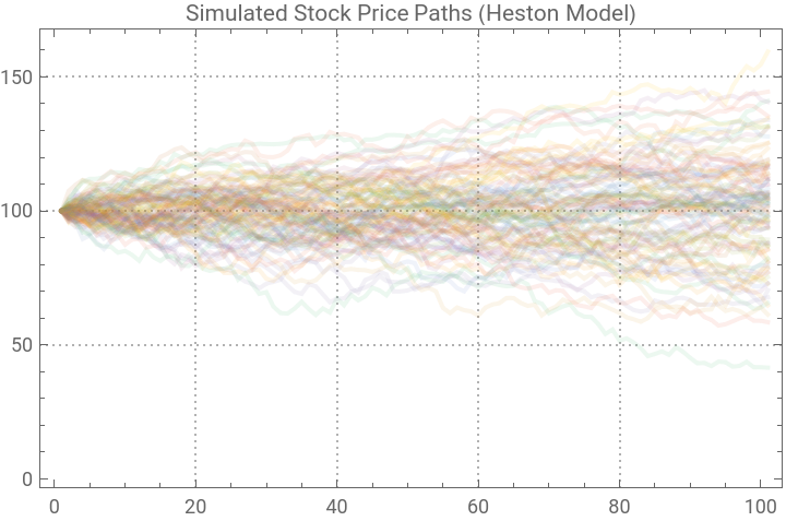
In[]:=
variancePlot=ListLinePlot[variancePaths,PlotLabel->"Simulated Variance Paths (Heston Model)",AxesLabel->{"Time Step","Variance"},PlotTheme->"Detailed",PlotStyle->Opacity[0.1]]
Out[]=
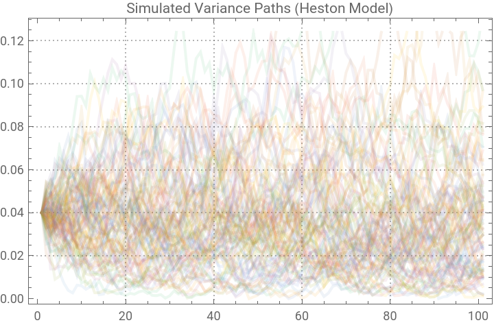
In[]:=
meanStockPath=Mean[stockPaths];meanVariancePath=Mean[variancePaths];
In[]:=
%471
Out[]=
{100,99.7634,100.139,100.364,100.059,99.8702,99.6189,99.7958,99.8559,100.054,99.9499,99.8784,100.089,99.9629,100.258,100.411,99.9698,100.135,100.171,100.207,100.013,100.141,99.9294,100.104,100.208,100.322,100.343,99.8456,99.8176,99.6878,99.3381,99.3035,99.3659,99.4262,99.4195,99.6249,99.6085,99.4967,99.2321,99.1012,99.2671,99.532,99.6438,99.8096,99.9303,100.132,100.338,100.474,100.453,100.405,100.565,100.446,100.332,100.259,100.396,100.387,100.508,100.162,100.136,100.271,100.203,100.405,100.741,100.769,100.728,100.975,101.069,101.098,101.29,101.262,101.285,101.13,101.066,101.156,101.318,101.312,101.694,101.41,101.382,101.161,101.049,101.377,101.557,101.121,101.28,101.212,101.146,101.307,101.382,101.463,101.169,101.243,101.103,101.155,100.997,101.126,101.225,101.289,101.308,101.378,101.807}
In[]:=
meanStockPlot=Show[ListLinePlot[stockPaths,PlotStyle->Opacity[0.1]],ListLinePlot[meanStockPath,PlotStyle->{Thick,Red}],PlotLabel->"Mean Stock Price Path (Heston Model)",AxesLabel->{"Time Step","Stock Price"},PlotTheme->"Detailed"]
Out[]=
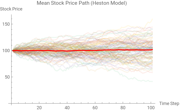
In[]:=
meanVariancePlot=Show[ListLinePlot[variancePaths,PlotStyle->Opacity[0.1]],ListLinePlot[meanVariancePath,PlotStyle->{Thick,Red}],PlotLabel->"Mean Variance Path (Heston Model)",AxesLabel->{"Time Step","Variance"},PlotTheme->"Detailed"]
Out[]=
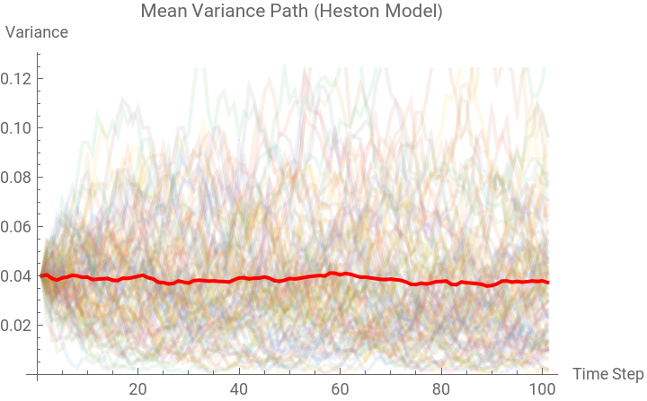
In[]:=
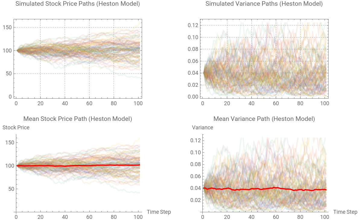
GraphicsGrid[{{stockPlot,variancePlot},{meanStockPlot,meanVariancePlot}}]
Out[]=
Option Pricing
Option Pricing
In[]:=
K=100;
In[]:=
callPrices=Max[#[[-1]]-K,0]&/@stockPaths;
In[]:=
estimatedCallPrice=Exp[-r*T]*Mean[callPrices];Print["Estimated Call Option Price: ",estimatedCallPrice]
Estimated Call Option Price: 8.86573
Distribution Analysis
Distribution Analysis
In[]:=
Histogram[stockPaths[[All,-1]],PlotLabel->"Distribution of Final Stock Prices",AxesLabel->{"Stock Price","Frequency"},PlotTheme->"Detailed"]