Wolfram Cloud Document

ABSTRACT: Hyperbolic lattices present a unique opportunity to venture beyond the conventional paradigm of crystalline many-body physics and explore correlated phenomena in negatively curved space. As a theoretical benchmark for such investigations, we extend Kitaev’s spin-1/2 honeycomb model to hyperbolic lattices and exploit their non-Euclidean space-group symmetries to solve the model exactly. In this Wolfram Mathematica notebook, we first show how to construct Kitaev models on hyperbolic lattices. Subsequently, we demonstrate how to use hyperbolic band theory to obtain the ground-state phase diagram on one of them and study the phases therein. In particular, we study the exotic compressible spin liquid with low-energy density of states dominated by non-Abelian Bloch states of Majorana fermions appearing for isotropic couplings which develops into a gapped chiral spin liquid under a time-reversal-breaking perturbation. CITATION (original article): Lenggenhager, P. M., Dey, S., Bzdušek, T., and Maciejko, J. Hyperbolic Spin Liquids. Phys. Rev. Lett. Accepted (2025). https://doi.org/10.1103/s25y-s4fj
arXiv: https://doi.org/10.48550/arXiv.2407.09601
DATA & CODE REPOSITORY: Lenggenhager, P. M., Dey, S., Bzdušek, T., and Maciejko, J. Supplementary data and code for: Hyperbolic Spin Liquids. Zenodo (2025). https://doi.org/10.5281/zenodo.14439718

Hyperbolic Kitaev model

We generalize Kitaev’s honeycomb model for quantum spin liquids [A. Kitaev, Anyons in an exactly solved model and beyond, Ann. Phys. 321, 2 (2006)] to hyperbolic

{p,3}

lattices. In general, the Kitaev model requires a 3-coordinated graph together with a 3-edge coloring of its edges (which does not necessarily exist). The 3-edge coloring assigns one of three colors to each edge such that the three edges adjacent to each vertex are distinct. Given these two objects, the model on the graph is defined by the Hamiltonian



-

∑

〈j,k〉



-K

∑

[lmn]

αβγ



where the sum in the first term runs over all edges of the graph with

specifying its color according to the 3-edge coloring and the sum in the second term runs over counterclockwise-oriented triplets of vertices

n,m,l

(denoted

[lmn]

αβγ

) that are connected by bonds

〈l,m〉

and

〈m,n〉

. The totally antisymmetric tensor

αβγ

satisfies

xyz

+1

and

β≠α,γ

is the color of the third bond adjacent to site

Model definition using HyperCells and HyperBloch

Conveniently, we define the model in translation-invariant fashion directly on a primitive cell of the hyperbolic

{p,3}

lattices under investigation, which can be easily done using the HyperCells [https://doi.org/10.5281/zenodo.10782370] and HyperBloch [https://doi.org/10.5281/zenodo.10783024] packages, which include a library of unit cells for hyperbolic lattices based on the following references: M. Conder, Quotients of triangle groups acting on surfaces of genus 2 to 101 (2007), https://www.math.auckland.ac.nz/~conder/TriangleGroupQuotients101.txt.

Installation

To install the HyperBloch package (and its dependency NCAlgebra) from Github, execute the following commands:

PacletInstall["https://github.com/NCAlgebra/NC/blob/master/NCAlgebra-6.0.3.paclet?raw=true"];PacletInstall["https://github.com/patrick-lenggenhager/HyperBloch/releases/download/v1.0.2/PatrickMLenggenhager__HyperBloch-1.0.2.paclet"];

Please note that NCAlgebra version ≥ 6 is required due to breaking changes in their implementation.

Primitive cell

First, load the package:

In[]:=

Needs["PatrickMLenggenhager`HyperBloch`"]

We consider the case of a single (primitive) unit cell of the

{8,3}

-lattice, i.e., the hyperbolic lattice with three octagons touching at each site. The output of HyperCells is the text file with the following content, which is shipped as an example with HyperBloch:

In[]:=

cellgraphT21=ImportCellGraphString[Import["PatrickMLenggenhager/HyperBloch/ExampleData/(2,3,8)_T2.1_3.hcc"]];

Next, we need the model graph defining the adjacency graph of the

{8,3}

-lattice (rather than the one of all maximally-symmetric Wyckoff positions):

In[]:=

modelgraphT21=ImportModelGraphString[Import["PatrickMLenggenhager/HyperBloch/ExampleData/{8,3}-tess_T2.1_3.hcm"]];

VisualizeModelGraphmodelgraphT21,



Out[]=

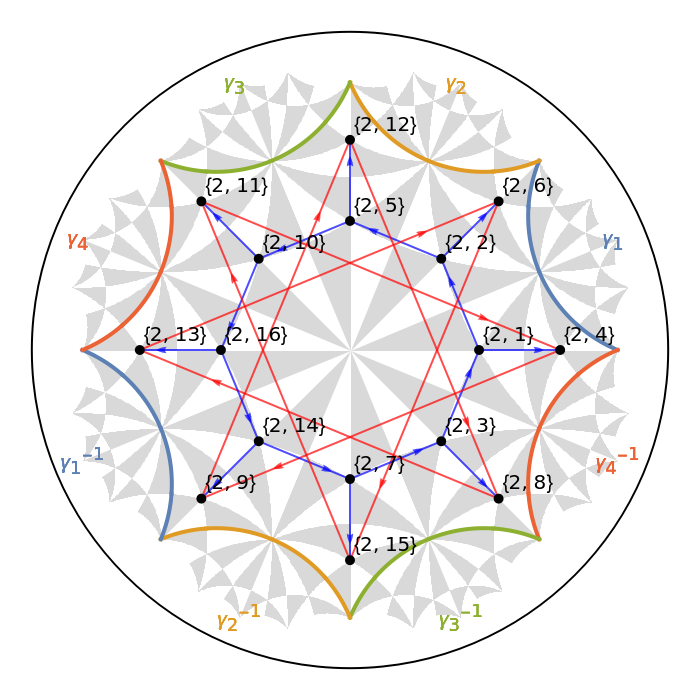
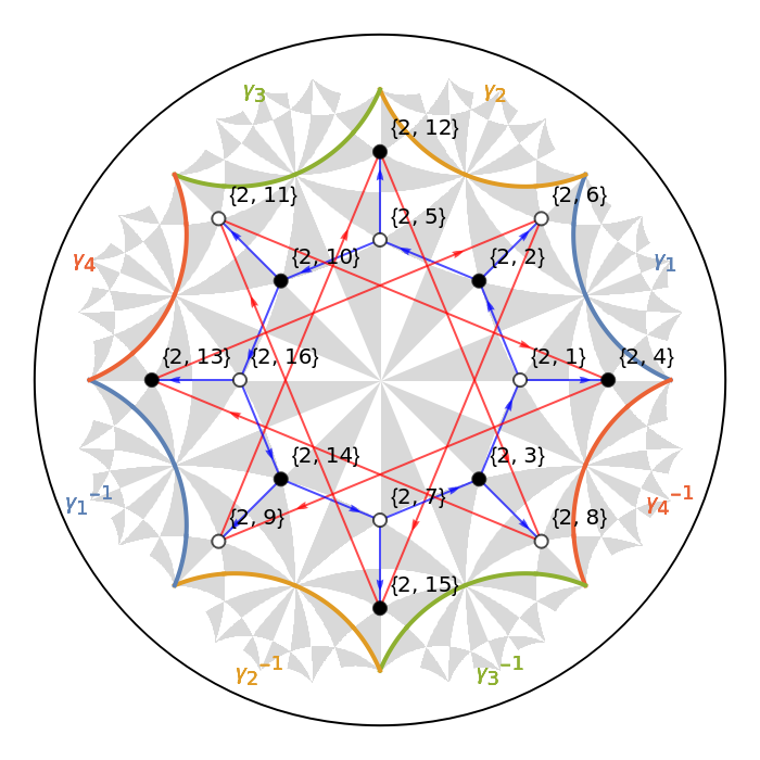
With

p8

even, the graph is bipartite, such that we can identify two sublattices or equivalently a 2-vertex coloring:

In[]:=

sublats=AssociationThread[VertexList[modelgraphT21["Graph"]]->FindVertexColoring[modelgraphT21["Graph"]]]

Out[]=

{2,1}2,{2,2}1,{2,3}1,{2,4}1,{2,5}2,{2,6}2,{2,7}2,{2,8}2,{2,9}2,{2,10}1,{2,11}2,{2,12}1,{2,13}1,{2,14}1,{2,15}1,{2,16}2

which we visualize as follows:

VisualizeModelGraphmodelgraphT21,



Out[]=

We next need to assign colors to all edges in the unit cell appropriately.

Finding arbitrary colorings compatible with translation symmetry

An arbitrary 3-edge coloring can be found using the Mathematica function FindEdgeColoring:

In[]:=

coloring=AssociationThread[EdgeList[modelgraphT21["Graph"]]->FindEdgeColoring[modelgraphT21["Graph"],{1,2,3}]];coloring=Join[coloring,Association@KeyValueMap[DirectedEdge[#1[[2]],#1[[1]],-#1[[3]]]->#2&,coloring]];

colors={

};VisualizeModelGraphmodelgraphT21,



Out[]=

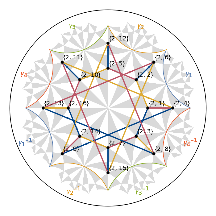
Since the number of edges per face, 8, is not divisible by the number of colors, 3, the typical coloring employed in the original honeycomb version of the model [A. Kitaev, Anyons in an exactly solved model and beyond, Ann. Phys. 321, 2 (2006)] is not possible. The coloring found above, has the following structure:

In[]:=

Counts[Values@KeySort@Counts[coloring[#]&/@EdgeList@Subgraph[modelgraphT21["Graph"],#]]&/@modelgraphT21["Faces"]]

Out[]=

{3,3,2}2,{2,3,3}2,{3,2,3}2

where the association counts how many times each type of face occurs and the face is characterized by the number of times each of the three colors occurs.

Note that, by construction, the coloring is always compatible with translation symmetry on the infinite hyperbolic lattice.

Symmetric coloring

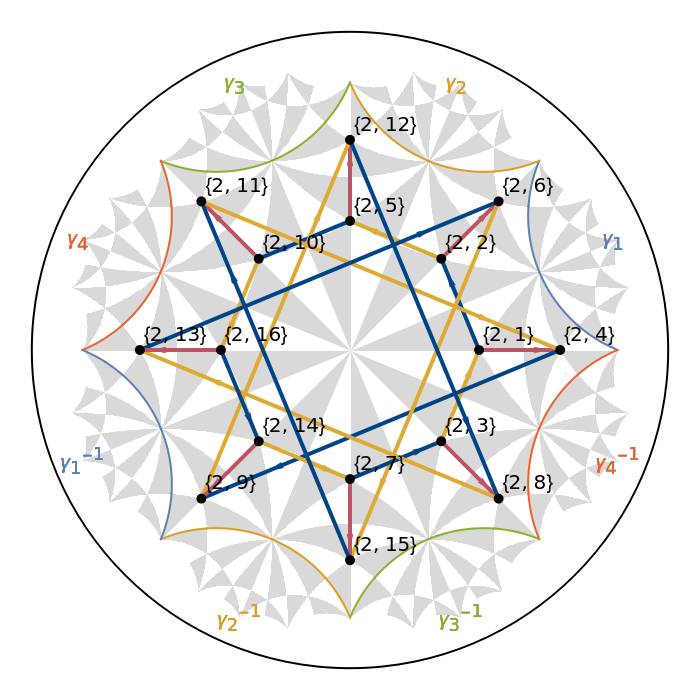
In our original article, we construct a specific coloring that is maximally symmetric and prove its existence on infinite hyperbolic

{p,3}

lattices (with

even) as well as unit cells specified by a translation group

Γ⊲Δ(p/2,p/2,p/2)

. For

p8

, we find the following coloring:

coloringSymmetric=

;

VisualizeModelGraphmodelgraphT21,



Out[]=

Exact solution

Majorana representation

With this, we verify that our choice indeed corresponds to no fluxes:

Note that we do not care about the Wilson loops along incontractible loops that exist the in the primitive cell when interpreted as a finite graph, since we assume it to tile the infinite lattice.

We can also go the other way round and define a function that finds an arbitrary configuration for a given set of plaquette fluxes:

Implementation of the Majorana Hamiltonian

Before we can implement the Majorana Hamiltonian, in particular the second term, we need to know the correction orientation of next-nearest neighbor hoppings. First, this requires the graph with the corresponding (oriented) edges, which can be obtained using the HyperCells package:

As an example, let us consider the following next-nearest-neighbor edge:

then, we obtain the corresponding two nearest-neighbor edges:

Finally, we can define the hoppings appearing in the Majorana Hamiltonian

which allows us to easily construct the corresponding Abelian Bloch Hamiltonian from (Abelian) hyperbolic band theory J. Maciejko and S. Rayan, Hyperbolic band theory, Sci. Adv. 7, abe9170 (2021)] using

Phase diagram and compressible spin liquid

Supercell method

Note that in the original article, we work with larger supercells.

Determining the spectral gap in the thermodynamic limit

From previous works [R. Mosseri and J. Vidal, Density of states of tight-binding models in the hyperbolic plane, Phys. Rev. B 108, 035154 (2023), P. M. Lenggenhager, et al., Non-Abelian hyperbolic band theory from supercells, Phys. Rev. Lett. 131 , 226401 (2023),
T. Tummuru, et al., Hyperbolic non-Abelian semimetal, Phys. Rev. Lett. 132, 206601 (2024)], we know that spectral gaps obtained from Abelian hyperbolic band theory, either applied to primitive or supercells, do not always agree with the results in the thermodynamic limit. However, we have shown that the supercell method converges to that limit [P. M. Lenggenhager, et al., Non-Abelian hyperbolic band theory from supercells, Phys. Rev. Lett. 131 , 226401 (2023)]. Thus, instead of simply computing the gap on the largest supercell, we compute the density of states for the sequence of supercells and extrapolate it to the thermodynamic limit. We then define the spectral gap as the energy interval in which the extrapolated density of states vanishes.

As an example, we consider the point

First, we construct the Abelian Bloch Hamiltonian for each supercell

and then randomly sample the corresponding momenta to obtain the density of states

While the more sophisticated extrapolation procedure discussed in our publication requires more supercells to work and can give us proper error estimates, we can use the simplified version to just obtain an estimate of the gap. This simplified method determines the gap by the crossing of the integrated density of states. We thus, first define a function for integrating the discretized density of states data:

which results in the following much smoother curves:

This allows us to easily determine the intersection between the T17.2 and T5.1 curves using the function

Phase diagram of the spectral gap

By repeating the above calculations throughout the phase diagram, we obtain the following result:

Again, we start by constructing the Abelian Bloch Hamiltonian for each supercell

and then randomly sample the corresponding momenta to obtain the density of states

Gapped chiral spin liquid

Spectral gap

Chern number

In the Euclidean case, the gapped phase near the isotropic point is characterized by a nonzero Chern number [A. Kitaev, Anyons in an exactly solved model and beyond, Ann. Phys. 321, 2 (2006)]. Here, we show that the same is true on the hyperbolic lattice. However, due to the noncommutative translations, we cannot compute the Chern number in momentum space and instead need to compute it in real space. To achieve this, we use the real-space formula discussed by Kitaev as well [A. Kitaev, Anyons in an exactly solved model and beyond, Ann. Phys. 321, 2 (2006)] which applies even to disordered systems. Since this is a topological effect, we do not expect the embedding to affect the result, such that we simply work with the projected coordinates of the site in the hyperbolic lattice. The real-space Chern number is given by

Again, we start by constructing the Abelian Bloch Hamiltonian for the supercell

and the Chern number subsequently using the function

This calculation is sufficiently fast to compute the full phase diagram, in which case we compile the Hamiltonian expression as a function of the coupling strengths rather than momenta:

Conclusion

In this post, we demonstrated how to extend the Kitaev model for spin liquids to hyperbolic lattices, in particular utilizing the HyperCells and HyperBloch packages and capabilities of Mathematica. We subsequently utilized the supercell method to efficiently estimate the density of states and fermionic spectral gap in the thermodynamic limit in order to obtain phase diagrams. Finally, we used Kitaev’s real-space formulation of the Chern number to compute the phase diagram of the Chern number on a small PBC cluster corresponding to a symmetrized supercell. For a discussion of the physics of the model and the implications of our results, please have a look at the original publication [P. M. Lenggenhager, et al., Hyperbolic Spin Liquids. Phys. Rev. Lett. Accepted (2025). DOI: https://doi.org/10.1103/s25y-s4fj ], whose open-access version can be found here: https://patrick-lenggenhager.github.io/publications.html.

CITE THIS NOTEBOOK

Hyperbolic Spin Liquids
by Patrick M. Lenggenhager, Santanu Dey, Tomáš Bzdušek, and Joseph Maciejko
Wolfram Community, STAFF PICKS, August 11, 2025
https://community.wolfram.com/groups/-/m/t/3528683