Protein folding arises from the interplay between sequence, geometry, and energetics. This essay explores how much of that behavior can be reproduced with a minimal discrete polymer model in two dimensions and provides an extendable framework for implementing these models. Conformations are encoded as local turns along a linear sequence and connected through allowed single-step transformations to form a state-space graph. Different sequence alphabets, turn angles and state transition rules are compared. The resulting models generate diverse motifs and strongly sequence-dependent energy landscapes.
1. Motivating a Minimal Model
1. Motivating a Minimal Model
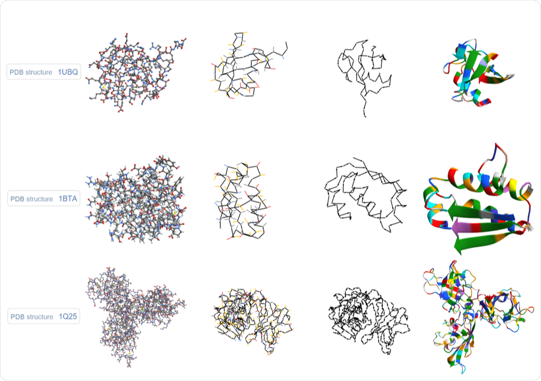
Shown below are structures of three proteins, each shown at four different resolutions. The first plot is at atom-level resolution. The second is at residue-level resolution, showing the backbone traced through the consecutive C-α atoms, with short branches in C-β direction to indicate the side-chains. (Side-chains being colored by broad side-chain type.) The third plot ignores side-chains entirely and keeps only the backbone. The fourth plot is a standard stylized representation of the third, backbone-trace plot, highlighting so-called secondary structure elements, foremost: helical arrangements of the backbone and sheets - where backbone segments align in parallel. Across these different resolutions, the core character of the structure is most apparent at the lower resolutions, capturing the global fold. Not only are proteins, outside of crystals, not static structures, the broad global fold contains enough information, to easily instantiate valid atomic resolution structures, as they could fleetingly appear in vivo.
Additionally, the apparent robustness with which different instances of the same protein arrive at the same global fold, as well as even different sequences, showing the same secondary structure features, or even the same global fold, suggests that the phenomenon is rather independent of the specific fine-grained bumps and vibrations a protein will go through during the folding process. This also suggests that it can be modeled at a more coarse resolution. Another interesting point is that some proteins tend to have rather long folding times, stretching multiple minutes, suggesting that a lot of sampling is involved in a protein finding its fold.
Additionally, the apparent robustness with which different instances of the same protein arrive at the same global fold, as well as even different sequences, showing the same secondary structure features, or even the same global fold, suggests that the phenomenon is rather independent of the specific fine-grained bumps and vibrations a protein will go through during the folding process. This also suggests that it can be modeled at a more coarse resolution. Another interesting point is that some proteins tend to have rather long folding times, stretching multiple minutes, suggesting that a lot of sampling is involved in a protein finding its fold.
Out[]=
To the extent that an organic molecule can be regarded as a graph, determining its structure is the problem of finding an embedding of that graph. Looking at the (heavy atom) molecule graph of Ubiquitin below, we again see that it is quite linear, with side-chains being only short branches of that graph.
Out[]=

So, proteins are linear chains of usually hundreds of amino acids and thousands of atoms. We can visualize them at different levels of detail, with the core characteristics arguably being the most apparent at the lowest (reasonable) resolutions, which naturally raises the question of how far we can push this while still retaining the qualitative properties. The most abstract version of this is to simply look at discrete embeddings of linear sequences. Historically these are called "Protein Lattice Models" with the "HP-model" being the most common version.
The point being that now whenever we find an interesting phenomenon we don't need to worry about what complicated combination of physical effects causes it, since all of what our model does is perfectly well defined.
The point being that now whenever we find an interesting phenomenon we don't need to worry about what complicated combination of physical effects causes it, since all of what our model does is perfectly well defined.
2. Model Setup
2. Model Setup
We will focus on short sequences where we can look at the entirety of state-space.
A model will be specified by a monomer sequence, a set of possible local orientations, rules for moving between them, and an energy function defined on the resulting conformations.
2.1 Encoding a Conformation
2.1 Encoding a Conformation
A state is represented by a list like {0,1,1,0,-1} that represents a sequence of rotation states between vertices. These are basically internal coordinates.
Together with an angle specification AnglePath will generate the corresponding Cartesian coordinates.
In[]:=
AnglePath[90Degree*{0,1,-1,0,-1}]
Out[]=
{{0,0},{1,0},{1,1},{2,1},{3,1},{3,0}}
2.2 Local Moves and the State-Space Graph
2.2 Local Moves and the State-Space Graph
In[]:=
ReplaceList[{0,0,1,0,-1},{{before__,0,after___}->{before,-1,after},{before__,0,after___}->{before,1,after},{before__,1,after___}->{before,0,after},{before__,-1,after___}->{before,0,after}}]
Out[]=
{{0,-1,1,0,-1},{0,0,1,-1,-1},{0,1,1,0,-1},{0,0,1,1,-1},{0,0,0,0,-1},{0,0,1,0,0}}
The first entry is fixed at 0, since it specifies the direction of the first edge from the vertex placed at the origin. Fixing this direction removes the otherwise irrelevant global rotation of the conformation.
Each resulting list differs from the original state at exactly one position. Repeatedly applying these local moves generates a graph whose vertices are conformations and whose edges represent allowed single-step transformations.
Out[]=
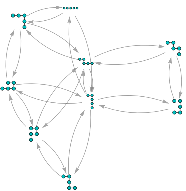
Since every allowed transformation in this example is accompanied by its reverse, the state-space graph can be displayed with undirected edges.
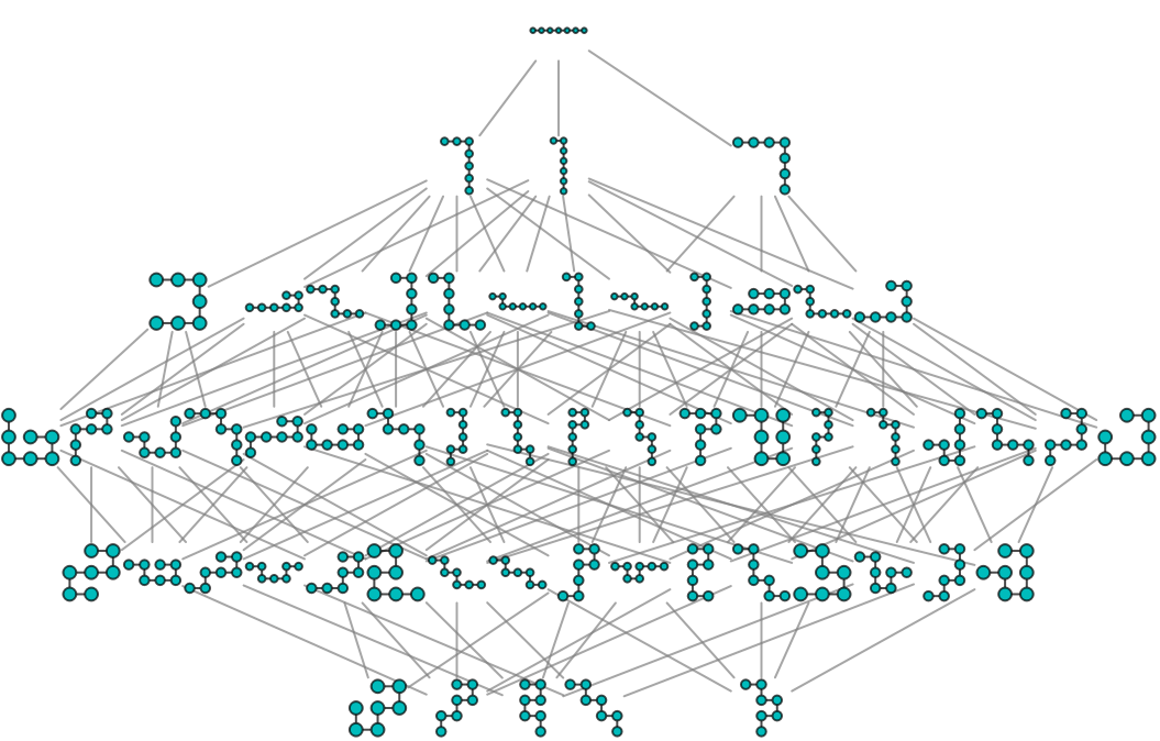
For length 7 the entirety of the state space looks like this:
Out[]=
2.3 Symmetry Reduction and Self-Avoidance
2.3 Symmetry Reduction and Self-Avoidance
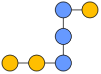
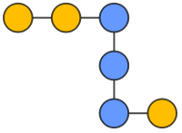
Different state lists can describe conformations that differ only by reflection or by reversing the direction in which the chain is read. These representations are treated as equivalent, and one canonical representative is retained for each equivalence class.
Out[]=
,
,
,
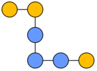
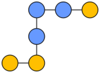
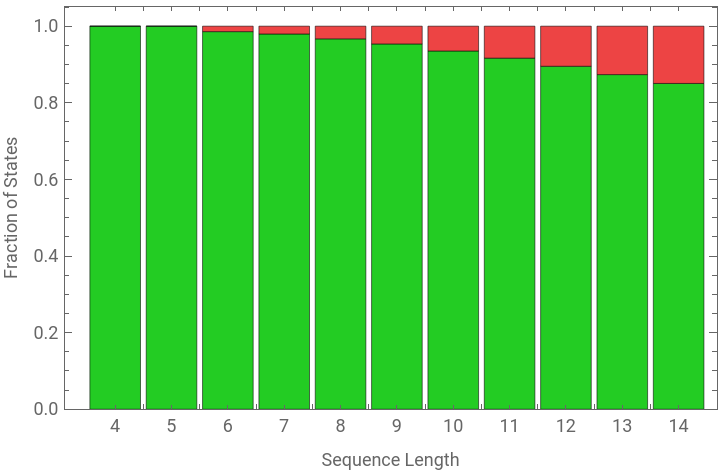
States in which two nonidentical vertices occupy the same Cartesian coordinates are excluded. The remaining conformations are therefore self-avoiding.
Out[]=


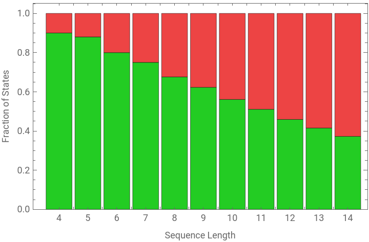
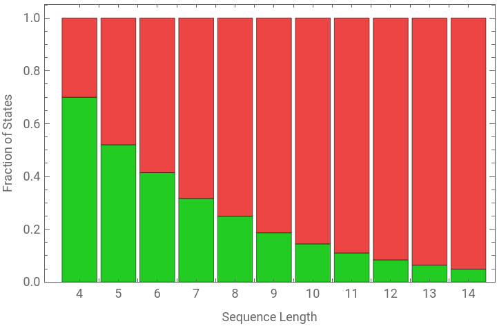
2.4 Sequence Types, Angles, and Interaction Energies
2.4 Sequence Types, Angles, and Interaction Energies
Along with the Uniform case, we already encountered, where all vertices are assumed to be the same, we will look at two additional kinds of sequences. “H | P” sequences, where the “H” stands for hydrophobic and the “P” stands for polar and “H | + | -” sequences where we split the polar case into positive and negative.
The following color codes are used:
Pairwise interaction terms used:
Note that the {H, H} (hydrophobic) interaction term is - 1 and the {P, P} (polar) interaction term is 0 even though hydrophobic interactions don’t intrinsically contribute energy, that they are favorable is a second order effect from them exposing a smaller total hydrophobic surface area to the surrounding water molecules that have favorable interactions. Here we factor out the to be assumed polar environment in this way.
2.5 Putting the Model Together
2.5 Putting the Model Together
The sequence, geometric rules, energy function, and other model specifications are collected in a PolymerModel object. This provides a common interface for constructing state spaces and accessing derived properties.
We start by examining a number of different states graphs for different “TurnAngle” and “StateTransitionRule” specifications, before we go on to look at energy distributions.
3. Resulting Geometries from Different Local Angle Rules
3. Resulting Geometries from Different Local Angle Rules
A slightly bigger example involving the same angle and state transition rules:
(Some of the labels are overlapping.)
(Some of the labels are overlapping.)
The most interesting shapes we see here probably are:
We see some interesting globular motifs:
Meandering motifs,
that also appear in combination with straight lines:
Unsurprisingly, as it allows a wider variety of angles along the chain, this is the most interesting case so far.
Giving us different globular arrangements:
Parallel chain alignments, which for this sequence also are our lowest energy configurations:
Meandering patterns,
as well as combinations thereof:
Other interesting motifs:
4. Energy Landscapes
4. Energy Landscapes
4.1 Low Energy States
4.1 Low Energy States
The model specifications used in this entire section were:
“TurnAngle” -> 60 Degree with “StateTransitionRules”->{-1<->1,2<->1,-2<->-1}, “EnergyNeighborhood”->1
“TurnAngle” -> 60 Degree with “StateTransitionRules”->{-1<->1,2<->1,-2<->-1}, “EnergyNeighborhood”->1
Example of a states graph that also includes energies:
The plot below shows for all three color sequences of length 7, deduplicated under string reversal, their lowest energy, together with the number of states that have this energy. The bubble size indicates how many sequences have that combination of {min energy, min energy states count} overall.
It can be seen that the lower the minimum energy is the more likely it is that it is unique.
Below is a big grid of plots for such minimum energy conformations.
4.2 Energy Distributions
4.2 Energy Distributions
The plots below show complete energy distributions for several sequences of increasing length. Each bar counts how many geometrically distinct conformations have a particular energy, while the structures above the bars provide examples from the corresponding energy level.
Sequences were chosen at random with a uniform distribution over the sequence alphabet {“H”, “+”, “-”}.
The interaction radius used for calculating the energies was one.
Length 7 sequences:
Length 7 sequences:
These energy histograms are quite different.
Length 9 sequences:
Length 13 sequences:
As the number of states grows the distribution shapes become more similar, with usually quite sharp tails.
It appears to be quite common it to be the case that there is a unique lowest energy state.
There appears to be high variability in how many minimum energy states there are.
5. Stationary Distributions of an Energy-Biased Walk Through State Space
5. Stationary Distributions of an Energy-Biased Walk Through State Space
Having looked at energy distributions, the next step is to examine how those energies interact with the structure of the state space. The plot below shows a transition probability matrix for PolymerModel[“+-HHH+-H”,<|”TurnAngle”->60Degree,”StateTransitionRules”->{-1<->1,2<->1,-2<->-1}|>].
The transition probability matrix is obtained from the model’s state-space adjacency matrix by weighting each edge according to the energy difference between the two connected states and then normalizing each row.
The transition probability matrix is obtained from the model’s state-space adjacency matrix by weighting each edge according to the energy difference between the two connected states and then normalizing each row.
The weighting factor used is very close to the the energy difference deltaE itself:
State-Transition-Probability-Matrix for PolymerModel[“+-HHH+-H”,<|”TurnAngle”->60Degree,”StateTransitionRules”->{-1<->1,2<->1,-2<->-1}|>]:
This looks rather symmetrical with the exception of the lower right hand side.
Having this transition probability matrix we can now nestedly apply it to a number of starting states to explore how the state distribution changes over time.
The picture below is a very representative example of how these distributions tend to look like. The upper plot is an array plot where each row is a state distribution vector, time progressing from the top to the bottom. States that appear further to the right in the state vector are ones that are further away from the default start state the state graph gets initialized with, which is the “maximally unfolded” configuration. Unsurprisingly the lowest energy states are much closer to being “maximally folded”.
The lower plot shows the state distributions overlaid on a list plot. Despite the states graph being rather connected and the transition probabilities between states differing a lot it takes about 1500 steps until the distribution stops changing, when applied to a uniform initial distribution (thin blue line at around .01 in the bottom graph), with the highest-probability state usually accounting for 30–70% of the total probability mass.
The lower plot shows the state distributions overlaid on a list plot. Despite the states graph being rather connected and the transition probabilities between states differing a lot it takes about 1500 steps until the distribution stops changing, when applied to a uniform initial distribution (thin blue line at around .01 in the bottom graph), with the highest-probability state usually accounting for 30–70% of the total probability mass.
Another example with a random length 8 sequence:
Presumably the states that still show “activity” after hundreds of steps are also rather close to each other in the states graph.
6. Local Rule Programs for Structural Transformation
6. Local Rule Programs for Structural Transformation
Sequences and states can be riffled together, making them suitable for overlapping neighborhood-rule replacements that update the central state. This makes it possible to study programs that operate directly on the data structures of the models we have looked at.
Example of a sequence and state being riffled together:
Example of a state progression as produced by a random program of this kind, red squares highlight overlapping states:
7. Usage and Implementation
7. Usage and Implementation
Concluding Remarks
Concluding Remarks
The models examined here are deliberately too simple to reproduce the detailed physics of real proteins. Their purpose is to isolate several structural ingredients of folding and make their consequences completely explicit. A conformation is generated from a finite sequence of local decisions, the allowed decisions determine the geometry of the state space and an interaction function assigns an energy to every state.
It has been observed that the resulting energy landscape is strongly sequence dependent, where for the same turn angles, state transition rules and sequence alphabet some sequences have a clearly distinguished minimum, while others possess many conformations of minimum energy. This also holds for nontrivial sequences.
The model was set up so that this could easily be studied on different sequence alphabets and different angles and transitions between them, as well as being easily extendable for future work. Branching sequences and the three-dimensional case will be interesting to look at, primarily because I expect helix- and sheet-like structure to be very common, given how simple they are. The implementation should also support using different angles and state transition rules between different vertices.
Acknowledgements
Acknowledgements
I would like to thank my mentors, Robert Nachbar and David DeBrota, for their helpful discussions and suggestions. I would also like to thank Stephen Wolfram for suggesting this project.
AI Disclosure
AI Disclosure
The following generative AI tool was used in this project:
ChatGPT 5.5 was used for brainstorming, debugging code and a small number of prose improvements. All code and written content was reviewed, understood and approved by the author.
ChatGPT 5.5 was used for brainstorming, debugging code and a small number of prose improvements. All code and written content was reviewed, understood and approved by the author.
CITE THIS NOTEBOOK
CITE THIS NOTEBOOK
Where Will It Settle? Exploring Polymer Folding with Minimal Discrete Models
by Christoph Steck
Wolfram Community, STAFF PICKS, July 16, 2026
https://community.wolfram.com/groups/-/m/t/3762337
by Christoph Steck
Wolfram Community, STAFF PICKS, July 16, 2026
https://community.wolfram.com/groups/-/m/t/3762337