Overview
Overview
This notebook is a progress report on my project to develop Mathematica access to the Schwab developer API. I am currently working on the Market Data Production app as an individual developer. I made an earlier post showing how I was able to create functions with assistance from Grok AI. I am now in the process of testing and refining the initial functions the latest version is now in a package script which can be run with Needs[“SchwabAPI`”]. The code is attached as a supplement to this post. A simple way to test the functions is to use old notebooks with functions that used FinancialData[]; this notebook tests daily prices with OHLCV data. The advantage to using the API is that the data is near real time so it gets current day data.
Over the next few days I will post additional notebooks to show how the API can be used and will include updates to the code.
If anyone with a Schwab account is interested in using this interface, the first step is to use the link above to apply for access to the API. Once you get that set up, I will be happy to walk you through the appAuthorization[] function to create the token system on your computer, if you make a comment to this post
Initialization code
Initialization code
The data from the SchwabAPI is converted to the same format as FinancialData[], the code beyond this section was most;y written in 2022.
In[]:=
Needs["SchwabAPI`"]
In[]:=
apiTokens=Import[tokenFile,"RawJSON"];apiTokens=refreshTokens[apiTokens["refresh_token"],appKey,appSecret];
In[]:=
startDate=DatePlus[Today,{-15,"Year"}];
In[]:=
prices=getPriceHistory["SPY",apiTokens["access_token"],startDate,Today,periodType"year",period"20",frequencyType"daily"];If[prices===$Failed,Abort[]]
In[]:=
dayDS=Dataset[prices["candles"]][All,RotateRight[Keys@prices["candles"][[1]]]]/.bigint_Integer:>If[bigint>10^12,DateObject[FromUnixTime[bigint/1000,TimeZone->"America/New_York"],"Day"],bigint];
In[]:=
data={#1,{#2,#3,#4,#5,#6}}&@@@Values[Normal[dayDS]];data[[-1]]
Out[]=
,{564.73,568.38,562.38,566.76,60717270}
Structure of intraday volatility
Structure of intraday volatility
The logarithm of the ratio of the daily high price to the daily low price, Log[high/low], can be used as a measure of intraday volatility caused by trading which is mostly done by computers. As a random variable this measure fits a description for an extreme value type of random variable, and a sample over 15 years of daily events is well fit by a generalized extreme value distribution. But the data points are not independently distributed, so the distribution is only useful for probabilities over a whole 15-year block of time, not the next event. Using the measure applied to the basic time unit of a trading day captures the role of trading in the price formation process. Trading positions are opened in higher volumes at the regular session market open and they are closed at the end of the session. The Log[high/low] then represents the extreme range of the process, standardized so the absolute value of price over long time scales does not affect the magnitude of the measure. A 15 year interval is chosen so that it will be very likely to have at least one market crash in the data (usually there are two crashes), but with respect to technology changes, it may be a rather long interval.
For this notebook the SPY ETF is used as to represent overall U.S. equity market behavior. The measure can also be used on individual stocks where it will be sensitive to events like trading after quarterly earnings release events.
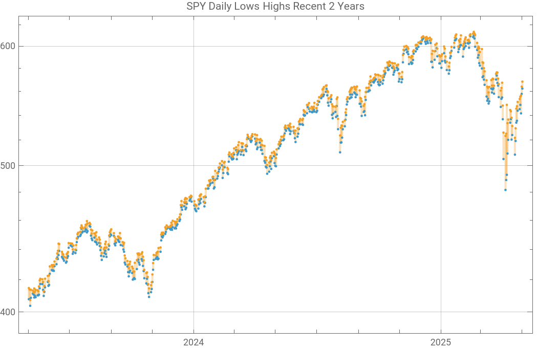
In the first graph below the blue and orange points are the daily low and high prices. The volatility graph is simply the log of the ratio of the high/low price each day.
In the first graph below the blue and orange points are the daily low and high prices. The volatility graph is simply the log of the ratio of the high/low price each day.
In[]:=
loghilo={#1,Log[#2[[2]]/#2[[3]]]}&@@@data;edf=EmpiricalDistribution[loghilo[[All,2]]];Last[loghilo][[2]]CDF[edf,%]
Out[]=
0.0106124
Out[]=
0.600689
In[]:=
q1=Quantile[edf,0.1]q5=Median[loghilo[[All,2]]]q9=Quantile[edf,0.9]
Out[]=
0.00440375
Out[]=
0.0090665
Out[]=
0.0208052
In[]:=
ygrid=Table[i,{i,0.01,Max[Take[loghilo[[All,2]],-252]]+0.01,0.01}]
Out[]=
{0.01,0.02,0.03,0.04,0.05,0.06,0.07,0.08,0.09,0.1,0.11}
Out[]=


Out[]=
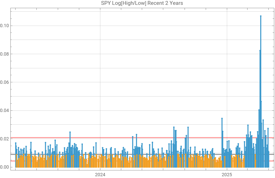
The 15 year median is the black line in the volatility chart. The red lines are the 0.1 and 0.9 quantiles. The peak price point of the SPY ETF occurred on 4 Jan 2022, a volatility spike occurred on 5 Jan 2022; since then U.S. equity markets have been in decline. Volatility has been above median for all but a few days since the volatility spike on 5 Jan. The rest of this notebook looks at the volatility signal in terms of run lengths above and below the median to see if the data contains any potentially useful information to predict the continuation or end of a run. The data set contains two previous market crashes; the current data could be the beginning of a third crash. The current economic factors are totally different from previous crash events, but financial markets have limited response patterns to information, i.e. prices can go up or down in varying magnitudes. Even though the economic parameters may be very different, price patterns will likely repeat.
Run lengths
Run lengths
The total number of days in the 15 year series.
In[]:=
Length[loghilo]
Out[]=
3774
Here a run consists of sequential volatility points either above or below the 15-year median.
In[]:=
runs=Split[loghilo,(#1[[2]]>=q5&[[2]]>=q5)||(#1[[2]]<q5&[[2]]<q5)&];
Probabiity of latest run length of volatility greater than median, if volatility were an independent random process.
In[]:=
runLengths=Length/@runs;%[[-1]]2^-%
Out[]=
27
Out[]=
1
134217728
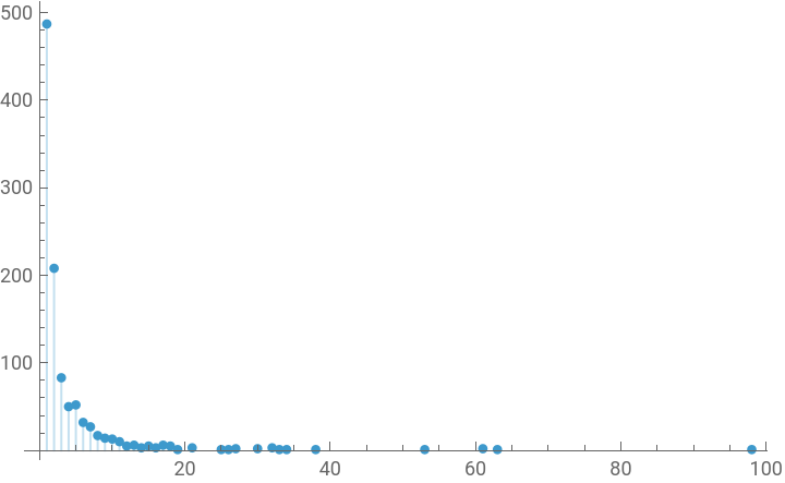
Long run lengths occur frequently.
In[]:=
runlen=Tally[runLengths]//SortListPlot[%,Filling->0,PlotRange->All]
Out[]=
{{1,487},{2,208},{3,83},{4,50},{5,52},{6,32},{7,27},{8,17},{9,14},{10,13},{11,10},{12,5},{13,6},{14,3},{15,5},{16,3},{17,6},{18,5},{19,1},{21,3},{25,1},{26,1},{27,2},{30,2},{32,3},{33,1},{34,1},{38,1},{53,1},{61,2},{63,1},{98,1}}
Out[]=
The longest run in the timeseries marked the end of the 2008 crash and beginning of the recovery. Notably after it ended equity markets rose for more than three years. Prior to this run breaking, volatility seemed to be generally declining.
In[]:=
longestRun=Select[runs,Length[#]==Max[runlen[[All,1]]]&][[1]];DateListPlotlongestRun,
Out[]=
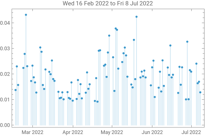
A listing of longer runs of volatility higher than median, including current run.
In[]:=
DateString[#[[1]][[1]],"DateShort"]<>" to "<>DateString[#[[-1]][[1]],"DateShort"]<>" Length "<>ToString[Length[#]]&/@Select[runs,Length[#]>=36&&#[[1]][[2]]>q5&]//TableForm
Out[]//TableForm=
Wed 3 Aug 2011 to Thu 27 Oct 2011 Length 61 |
Mon 31 Oct 2011 to Thu 22 Dec 2011 Length 38 |
Thu 20 Feb 2020 to Tue 19 May 2020 Length 63 |
Wed 16 Feb 2022 to Fri 8 Jul 2022 Length 98 |
Long runs of below median volatility are shorter.
In[]:=
DateString[#[[1]][[1]],"DateShort"]<>" to "<>DateString[#[[-1]][[1]],"DateShort"]<>" Length "<>ToString[Length[#]]&/@Select[runs,Length[#]>20&&#[[-1]][[2]]<=q5&]//TableForm
Out[]//TableForm=
Thu 3 Jan 2013 to Fri 1 Feb 2013 Length 21 |
Fri 31 Oct 2014 to Fri 5 Dec 2014 Length 25 |
Tue 3 Jan 2017 to Mon 20 Mar 2017 Length 53 |
Wed 6 Sep 2017 to Thu 30 Nov 2017 Length 61 |
Tue 5 Dec 2017 to Fri 12 Jan 2018 Length 27 |
Fri 3 Aug 2018 to Wed 19 Sep 2018 Length 33 |
Wed 16 Oct 2019 to Fri 29 Nov 2019 Length 32 |
This is the longest run of volatility below median in the series.
Long run lengths cluster.
Occurrence of run lengths greater than 25.
About 23% volatility points are in clusters of longer runs than 25 trading days.
In graph above the third and the current cluster contain short breaks in the cluster. Thus not every break in a long run signals the end of a period of high volatility, but a single point below median volatility marked the end of the other long runs of high and low volatility in the chart above.
Low volatility runs.
CITE THIS NOTEBOOK
CITE THIS NOTEBOOK
Volatility analysis using daily price data from the Schwab API
by Robert Rimmer
Wolfram Community, STAFF PICKS, May 4, 2025
https://community.wolfram.com/groups/-/m/t/3454679
by Robert Rimmer
Wolfram Community, STAFF PICKS, May 4, 2025
https://community.wolfram.com/groups/-/m/t/3454679