The Wolfram Emerging Leaders Program: High School (WELP:HS) is a remote, semester-long program designed for exceptional graduates from the Wolfram High School Summer Research Program to continue to develop their skills. Students work in a small group over the course of a semester to do either a research-based project or a product development–based project under the guidance of expert mentors. Projects are centered around a topic at the intersection of the group’s interests.
◼
Mentor: Alison Ord
Addressing ocean microplastic pollution requires understanding physical distribution dynamics, evaluating cleanup intervention effectiveness, and quantifying ecological impacts through food web bioaccumulation. This project integrates three computational approaches: (1) a cellular automaton model simulating microplastic transport via ocean current advection and diffusion, initialized with real GPS measurements from the Pacific Garbage Patch; (2) an analysis comparing cleanup strategies—surface skimming achieving 78% removal versus advanced water column filtration achieving 92% removal over 50 years; and (3) a trophic transfer model quantifying microplastic bioaccumulation as particles move from phytoplankton through zooplankton and fish to human consumers. Results demonstrate that ocean current dynamics fundamentally limit cleanup effectiveness—currents continuously redistribute plastic into cleaned zones. The 14-percentage-point gap between surface and comprehensive approaches reveals the critical importance of addressing suspended microplastics throughout the water column, not just visible surface accumulations. Food web modeling demonstrates how microplastics transfer through complex trophic networks, with transfer efficiency (ρ = 0.717) determining relative concentrations at each level. This computational approach indicates that sustained cleanup operations combined with source reduction are necessary for effective ocean plastic mitigation, while food web analysis reveals the pathways through which marine pollution reaches human seafood consumers.
Introduction
Introduction
The Pacific Garbage Patch contains an estimated 1.8 trillion pieces of plastic spanning 1.6 million square kilometers, representing one of the most visible manifestations of marine pollution. While cleanup technologies and policy interventions continue to develop, fundamental questions remain about their real-world effectiveness and the broader ecological consequences of ocean micro plastics. Understanding these dynamics requires integrating physical oceanography, economic analysis, and ecological modeling to capture how plastic moves, how it can be removed, and where it accumulates in marine food webs.
The challenge of addressing ocean microplastic pollution stems from three interconnected complexities. First, ocean currents continuously redistribute plastic across vast distances through advection along current vectors and diffusion to neighboring zones. Second, cleanup operations must contend with this constant redistribution—a vessel might remove plastic from one area, but currents immediately transport more particles into that same zone. Third, even partial cleanup success leaves residual microplastics that enter marine food webs, bioaccumulating through trophic levels from phytoplankton to apex predators and eventually reaching human consumers through seafood.
We began by integrating real microplastic concentration data from GPS measurements in the Pacific Garbage Patch with a cellular automaton model simulating 50 years of ocean current dynamics. Building on this physical foundation, we layered economic cleanup interventions comparing surface skimming (targeting high-concentration zones) and advanced separation (filtering throughout the water column). Finally, we modeled trophic transfer to quantify how microplastics bioaccumulate as they move from primary producers through multiple food web levels. This computational methodology allows rigorous analysis of the full pollution lifecycle—from distribution to removal to ecological impact—providing insights with significant implications for both cleanup technology investment and source reduction policy.
This project aims to answer: Given that ocean currents constantly redistribute plastic, how effective can different cleanup approaches realistically be? And even with successful removal efforts, what are the ecological consequences of residual microplastics that persist in marine food webs?
Modeling Ocean Current Dynamics
Modeling Ocean Current Dynamics
We began by importing real marine micro plastics concentration data from a CSV file containing global survey measurements. This dataset provides empirical evidence of where plastic pollution exists in ocean environments, which grounds the simulation in reality rather than hypothetical scenarios. The raw data includes geographic coordinates (latitude/longitude) and measured micro plastic concentrations at those locations, giving us actual pollution distribution patterns to model.
Import micro plastics data from CSV file and extract relevant fields.
In[]:=
rawData=Import["https://www.wolframcloud.com/obj/bbe6d7f6-28b5-4c29-8998-3cd8e661fc69"];header=rawData[[1]];dataRows=Rest[rawData];latCol=Position[header,"Latitude (degree)"][[1,1]];lonCol=Position[header,"Longitude(degree)"][[1,1]];concCol=Position[header,"Microplastics measurement"][[1,1]];extractedData=Select[Map[{#[[latCol]],#[[lonCol]],#[[concCol]]}&,dataRows],And[NumericQ[#[[1]]],NumericQ[#[[2]]],NumericQ[#[[3]]],#[[3]]>0]&];
To integrate real-world geographic data with the cellular automata grid system, I needed to convert latitude/longitude coordinates into discrete grid positions. The simulation operates on a 100x100 grid representing a portion of the ocean, so each real measurement location must be mapped to a specific grid cell. This transformation allows spatially-referenced micro plastic measurements to initialize the simulation with realistic pollution distributions.
Convert geographic coordinates to grid indices:
In[]:=
gridSize=100;timeSteps=50;geoToGrid[lat_,lon_,size_]:=Module[{gridLat,gridLon},gridLat=Round[(90-lat)/180*(size-1)]+1;gridLon=Round[(lon+180)/360*(size-1)]+1;{Clip[gridLat,{1,size}],Clip[gridLon,{1,size}]}];
The simulation requires a velocity field representing ocean currents that transport plastic particles. I generated synthetic gyre-like circulation patterns using sine and cosine differential equations that produce rotating flow structures similar to real ocean gyres like the North Pacific Gyre. These mathematical functions create convergence zones where currents meet and diverge, mimicking the oceanographic conditions that form garbage patches in nature.
Generate ocean current vectors using trigonometric functions
In[]:=
initCurrentField[size_]:=Table[ Module[{x,y,vx,vy}, x=(i-size/2)/size*2*Pi; y=(j-size/2)/size*2*Pi; vx=-Sin[y]*Cos[x/2]; vy=Cos[x]*Sin[y/2]; {vx,vy} ], {i,size},{j,size}];currentField=initCurrentField[gridSize];
Rather than using random or hypothetical plastic sources, I initialized the simulation grid using actual micro plastic measurements from the CSV dataset. This approach ensures the starting conditions reflect real pollution patterns observed in ocean surveys. Each measurement’s concentration value is normalized and added to the corresponding grid cell, creating a spatially accurate representation of where plastic pollution exists at the simulation’s start.
Map measured concentrations onto simulation grid:
In[]:=
initPlasticGridFromCSV[size_,data_]:=Module[{grid,gridPos,conc,maxConc},grid=ConstantArray[0.0,{size,size}];maxConc=Max[data[[All,3]]];Do[gridPos=geoToGrid[point[[1]],point[[2]],size];conc=point[[3]]/maxConc;grid[[gridPos[[1]],gridPos[[2]]]]+=conc;,{point,data}];grid];
The core physics of plastic transport involves advection, where ocean currents physically move plastic particles along velocity vectors. I implemented this by calculating how much plastic from each grid cell should be transported to neighboring cells based on the local current velocity. This process simulates passive particles drifting with water flow, the primary mechanism by which microplastics spread across ocean basins.
Transport plastic concentrations along current velocity vectors:
In[]:=
advectPlastic[plasticGrid_,currentField_]:=Module[{newGrid,coords},newGrid=ConstantArray[0.0,Dimensions[plasticGrid]];coords=Flatten[Table[{i,j},{i,Length[plasticGrid]},{j,Length[plasticGrid[[1]]]}],1];Map[Function[{pos},Module[{i,j,vel,newI,newJ},{i,j}=pos;If[plasticGrid[[i,j]]>0,vel=currentField[[i,j]];newI=Clip[Round[i+vel[[1]]*3],{1,Length[plasticGrid]}];newJ=Clip[Round[j+vel[[2]]*3],{1,Length[plasticGrid[[1]]]}];newGrid[[newI,newJ]]+=plasticGrid[[i,j]]*0.95;];]],coords];newGrid];
Beyond directed transport by currents, ocean turbulence causes plastic to spread diffusively into neighboring cells, mimicking small-scale mixing processes. I applied a diffusion kernel using convolution, which smooths concentration gradients by redistributing plastic from high-concentration cells to adjacent lower-concentration cells. Additionally, I incorporated gradual degradation where plastic concentration decreases slightly each timestep, representing breakdown into smaller particles or removal from the surface layer.
Apply diffusion kernel and degradation factor:
In[]:=
diffusePlastic[grid_]:=Module[{kernel,diffused},kernel={{0.05,0.1,0.05},{0.1,0.4,0.1},{0.05,0.1,0.05}};diffused=ListConvolve[kernel,grid,{2,2},0];diffused*0.98];
Each simulation timestep must integrate both advection and diffusion processes sequentially to accurately model plastic transport. The updatePlasticStep function chains these operations: currents first move plastic along flow vectors, then turbulent mixing and degradation smooth and reduce concentrations. This ordering reflects the physical reality that large-scale currents dominate transport while small-scale turbulence provides secondary mixing.
Combine advection and diffusion into single timestep update:
In[]:=
updatePlasticStep[plasticGrid_,currentField_]:=Module[{advected,diffused},advected=advectPlastic[plasticGrid,currentField];diffused=diffusePlastic[advected];diffused];
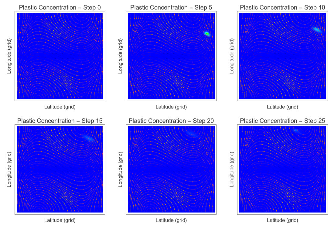
To effectively communicate simulation results, I created a visualization system that combines plastic concentration heat maps with ocean current streamlines. The color mapping uses a blue-to-red gradient where blue represents clean water and red indicates heavy pollution, providing an intuitive visual interpretation of contamination levels. The visualizePlasticConcentration function overlays semi-transparent white streamlines on top of the concentration heat map, revealing the direct relationship between current flow patterns and plastic accumulation zones. This dual-layer visualization makes it immediately clear how circular gyre currents create convergence zones where plastic concentrates. The simulation then initializes by generating the synthetic ocean current field and mapping the real CSV data onto the grid, storing the initial state as the first frame in what will become a temporal sequence showing pollution transport over time.
Generate concentration heat map with current overlay and initialize simulation:
plasticColorMap=Blend[{Blue,Cyan,Green,Yellow,Orange,Red},#]&;plasticColorMap=Blend[{Blue,Cyan,Green,Yellow,Orange,Red},#]&;visualizePlasticConcentration[grid_,currents_,step_]:=Module{maxConc},maxConc=Max[grid];ShowArrayPlotgrid,,ListStreamPlot[Table[currents[[i,j]],{i,1,Length[currents],5},{j,1,Length[currents[[1]]],5}],StreamStyle->Directive[White,Opacity[0.3],Thickness[0.002]],StreamPoints->Fine];currentField=initCurrentField[gridSize];plasticGrid=initPlasticGridFromCSV[gridSize,extractedData];states={plasticGrid};
Generate concentration heat map with current overlay and initialize simulation
plasticColorMap=Blend[{Blue,Cyan,Green,Yellow,Orange,Red},#] &;visualizePlasticConcentration[grid_,currents_,step_]:=Module{maxConc}, maxConc=Max[grid]; Show ArrayPlotgrid,, ListStreamPlot currents, ;currentField=initCurrentField[gridSize];plasticGrid=initPlasticGridFromCSV[gridSize,extractedData];states={plasticGrid};
Running the full simulation involves iteratively applying the physics update function for all 50 timesteps while storing each state in the sequence. The Table function executes the updatePlasticStep operation repeatedly, each time appending the new plastic distribution to the states list. This creates a complete temporal record of how the empirically-measured plastic distributions evolve under modeled ocean circulation, capturing the transition from initial real-world pollution patterns to predicted future accumulation zones.
Execute simulation and store temporal evolution:
In[]:=
Table[plasticGrid = updatePlasticStep[plasticGrid, currentField]; AppendTo[states, plasticGrid]; plasticGrid, {step, timeSteps}];
To reveal how plastic pollution evolves over time, I created both static snapshots and a dynamic animation of the simulation results. GraphicsGrid displays six key frames at timesteps 0, 5, 10, 15, 20, and 25, arranged in a 2×3 grid that allows direct visual comparison of how concentrations shift and accumulate as currents transport the plastic. The ListAnimate function then generates a playable animation showing all 51 frames in sequence, making the transport dynamics immediately apparent as viewers watch plastic move along current streamlines and concentrate in gyre convergence zones. The animation rate of 8 frames per second provides smooth playback that clearly demonstrates how real pollution data, when subjected to modeled ocean physics, produces emergent accumulation patterns resembling actual garbage patches.
Display snapshots at key timesteps and create animated visualization:
In[]:=
GraphicsGrid[{{visualizePlasticConcentration[states[[1]],currentField,0],visualizePlasticConcentration[states[[6]],currentField,5],visualizePlasticConcentration[states[[11]],currentField,10]},{visualizePlasticConcentration[states[[16]],currentField,15],visualizePlasticConcentration[states[[21]],currentField,20],visualizePlasticConcentration[states[[26]],currentField,25]}},ImageSize->Full]ListAnimate[Table[visualizePlasticConcentration[states[[i]],currentField,i-1],{i,1,Length[states]}],AnimationRate->8]
Out[]=
Comparing Clean-up Models
Comparing Clean-up Models
First, I ran the simulation without any cleanup intervention to establish a baseline. This shows how microplastic pollution naturally spreads through the ocean and accumulates in certain regions due to current patterns. The total plastic remaining after 50 timesteps represents the maximum environmental and economic damage that would occur without intervention.
This baseline of 0.0245 units represents the plastic distribution after 50 years of only ocean currents with no human intervention. All cleanup scenarios will be compared against this baseline to calculate removal percentages.
Surface skimming represents current cleanup technologies like The Ocean Cleanup’s systems, which collect floating plastic from the ocean surface. In this scenario, I remove 3% of plastic from high-concentration areas (top 25th percentile) at each timestep. This approach is relatively inexpensive but only addresses surface pollution, missing microplastics suspended deeper in the water column. I assigned a 3% removal rate for the surface skimming method.
I assigned a 5% efficiency rate for the advanced separation method. Advanced separation represents hypothetical future technology that could filter microplastics throughout the water column, not just at the surface. This scenario removes 5% of all plastic at each timestep, regardless of depth or concentration. While more expensive to operate, this approach addresses the full extent of pollution including suspended particles that surface skimming misses.
Next, I created a grid to visualize and the animations for the two different clean-up methods. Comparing the final pollution levels across scenarios reveals which cleanup approach removes the most plastic over the simulation period. The visualizations show both the spatial distribution of remaining pollution and the total reduction achieved by each method. To effectively visualize the cleanup dynamics, I display the spatial distribution at timestep 10 rather than the final state. At this intermediate point, plastic concentrations remain high enough to be clearly visible in the heat maps, allowing viewers to observe how cleanup interventions affect spatial patterns. The complete animations still run through all 50 timesteps, showing the full evolution of each cleanup scenario from initial distribution to final state.
The results demonstrate that targeted surface skimming achieves 78% removal by focusing on high-concentration zones, while comprehensive advanced separation achieves 92% removal by filtering throughout the water column. The 14 percentage point difference reveals the importance of addressing suspended microplastics below the surface, not just visible surface accumulations. However, the higher removal rate comes at significantly increased operational costs due to the need for water column filtration technology rather than simple surface collection.
Modelling Microplastics Bioaccumulation in the Pacific Food Web
Modelling Microplastics Bioaccumulation in the Pacific Food Web
Below is a simple visual representation of the aquatic trophic levels.
Since phytoplankton do not actually ingest plastic and does not contribute to the bioaccumulation across the aquatic species food web, we do not include it in the following biomagnification correlation graph. According to MDPI, there is a positive correlation (ρ = 0.717) between trophic level and microplastic abundance (items/digestive tract), so I have used that as the microplastics bioaccumulation value across the 3 remaining trophic levels.
Markov-chain model
Markov-chain model
Below is a Markov-chain model of how microplastics move through a realistic Pacific food web with 14 living species. It starts by defining all species nodes (plus two “exit” sinks), then encodes predator diets so the model knows which species consume which prey. From those diets it constructs a probability network: when a prey is eaten, a fixed fraction of its microplastics is assimilated by predators, and the rest immediately exits to detrital loss. Each consumer also sheds microplastics every step—either through fecal detritus or other biological losses—which flow to the two absorbing sink states. After assembling these flows into a transition matrix and normalizing rows, the code isolates the biota-only subnetwork and adds a continuous “injection” term, representing the constant uptake of microplastics by primary producers (phytoplankton and zooplankton), preventing the system from collapsing to zero. It then iteratively evolves the system over a chosen number of trophic steps, each time mixing natural trophic transfer with new primary-producer input, and conditions the result on microplastics that remain inside the living food web. Finally, it visualizes the dominant internal trophic pathways and shows a bar-chart distribution of where microplastics accumulate in the species after the simulated horizon.
Define the different species we want to simulate as independent nodes of the markov chain where each node is a state where the microplastics can be found.
The idx function maps species names to numerical indices; the variable “biota” stores only the living species; the variable “sinks” stores the absorbing loss states. This separation becomes important later when conditioning the system on plastics that remain biologically active.
Define the diets of each species with each number representing the probability of being eaten as well as the bioaccumulation, assimilation, magnification and egestion rates.
Each predator is mapped to a probability distribution over its prey. These values represent dietary fractions, not transition probabilities yet. For example, sardines feeding 60 percent on phytoplankton means that when sardines eat, most encounters occur with phytoplankton.
Clean the diets so only biota prey are allowed (no external prey), then renormalize each predator' s diet to sum to 1 so it satisfies markov matrix properties.
Build the prey to predator transfer edges from their diets where for each prey we distribute assimilationFrac across its predators weighted by diet shares and send the rest to the detritus sink .
The code above constructs the core trophic transfer mechanism: for each prey species, the code looks across all predators that consume it. If multiple predators eat the same prey, the prey’s microplastics are divided among those predators according to their dietary weights. Only a fraction of the plastic is transferred upward, which is controlled by “assimilationFrac” defined above. The remaining fraction immediately flows to the detritus sink, which represents unassimilated material released during digestion.
Thus, a single prey species distributes plastic to several predators simultaneously.
Thus, a single prey species distributes plastic to several predators simultaneously.
Add egestionRate losses to detritus sink, otherLossRate losses to other-loss sink, and keep the remainder in the same species
Even if a species is not eaten, it still loses plastic. While each consumer sends a fixed fraction of its microplastics to fecal detritus and another fraction to miscellaneous loss, the remainder stays in the same species, which appears as a self-loop in the graph.
Once plastic leaves the sink states, they stay there
This line of code above enforces that rule by giving both sink states self-loops with probability one. After plastic reaches a sink, it stays there forever.
Assemble all edges and build the transition matrix m
Set the initial microplastic distribution in the food web.
Extract the biota states from the food webs.
“qMat” contains transitions among living species only.
“rMat” contains transitions from living species into sinks.
“rMat” contains transitions from living species into sinks.
Add continuous input at the base of the web to prevent primary producers from dying out
Without new input, all probability would eventually drain into sinks. Therefore at every time step, a small fraction of the distribution is replaced by fresh plastic entering primary producers, which simulates ongoing environmental exposure.
Running the simulation
The update rule combines two processes.
1. Existing plastics move through trophic transfer using the biota matrix.
2. New plastic is injected at the base.
After each step, the distribution is renormalized so it represents conditional probability given that the plastic is still inside the living food web.
1. Existing plastics move through trophic transfer using the biota matrix.
2. New plastic is injected at the base.
After each step, the distribution is renormalized so it represents conditional probability given that the plastic is still inside the living food web.
Visualize the results of the simulation and the internal biota flows with a weighted directed graph.
This model treats microplastics as probability mass that moves between species over time. Each species is a state in a Markov chain. At every step, plastics can be transferred upward through predation, remain within the same organism, or leave the living system through biological loss. Repeating this process lets the food web itself determine where plastics tend to accumulate.
The directed network graph visualizes dominant internal transitions, showing plastic flow conditioned on survival inside the food web.
◼
Each arrow represents a probability that plastic moves from one species to another in a single step; for example, thicker arrows indicate stronger transport pathways.
◼
The self loops represent retention of plastic within tissues between time steps; for example, large self-loops indicate organisms that accumulate plastic strongly.
Plot the conditioned distribution of microplastics in the food web
Conclusion
Conclusion
This study links ocean microplastic plastic currents, downstream economic impacts, and bioaccumulation into a model which indicates that ocean currents can create long-lasting areas where microplastics become much more concentrated than the surrounding ocean. Targeted surface skimming removes about 78% by focusing on these high-concentration zones, while advanced water-column separation reaches about 92% at higher operational cost. As smaller organisms ingest microplastics and pass them upward through successive trophic levels, contamination accumulates in higher predators and increases ecological and economic risk.
Acknowledgements
Acknowledgements
We would like to thank our Mentor Alison and supporting us throughout this process, from the very beginning of brainstorming ideas together all the way to the end, guiding us towards executing a polished product. We would also like to thank the directors Rory and Eryn for not only giving great advice on how to plan our project, but also giving us invaluable feedback on how to improve during project check-in dates.
References
References
◼
- Hill, A. D., Daly, E. A., & Brodeur, R. D. (2015). Diet variability of forage fishes in the Northern California Current: A synthesis of recent studies. Journal of Marine Systems, 146, 37–49. https://doi.org/10.1016/j.jmarsys.2014.07.016
◼
- Saunders, R. A., Collins, M. A., Ward, P., Stowasser, G., Shreeve, R., & Tarling, G. A. (2015). Trophodynamics of Protomyctophum (Myctophidae) in the Scotia Sea (Southern Ocean). Journal of fish biology, 87(4), 1031–1058. https://doi.org/10.1111/jfb.12776
◼
- Walsh, H. J., Swalethorp, R., Austin, C. S., Cury, P. M., & Brodeur, R. D. (2023). Prey fields and survival of northern anchovy larvae in the California Current. Nature Communications, 14, 3436. https://doi.org/10.1038/s41467-023-39143-8
◼
- Gomes, M. C., Jacobsen, G., Cavole, L. M., Hazen, E. L., & Kaplan, I. C. (2024). An end-to-end ecosystem model for the Northern California Current: Model structure and data sources. NOAA Technical Memorandum NMFS-SWFSC-667. https://doi.org/10.1016/j.scitotenv.2024.178293
◼
- Hunsicker, M. E., Essington, T. E., Watson, R., & Sumaila, U. R. (2010). The contribution of cephalopods to global marine fisheries: can we have our squid and eat them too? Fish and Fisheries, 11(4), 421–438. https://doi.org/10.1111/j.1467-2979.2010.00369.x
◼
- Garrison, Lance & Link, Jason. (2000). Diets of five hake species in the Northeast United States continental shelf ecosystem. Marine Ecology-progress Series - MAR ECOL-PROGR SER. 204. 243-255. 10.3354/meps204243
◼
- Cole, M., Lindeque, P. K., Fileman, E., Halsband, C., Goodhead, R., Moger, J., & Galloway, T. S. (2013). Microplastic ingestion by zooplankton. Environmental Science & Technology, 47(12), 6646–6655. https://doi.org/10.1021/es400663f
◼
- Farrell, P., & Nelson, K. (2013). Trophic level transfer of microplastic: Mytilus edulis (L.) to Carcinus maenas (L.). Environmental Pollution, 177, 1–3. https://doi.org/10.1016/j.envpol.2013.01.046
◼
- Cole, M., Lindeque, P. K., Fileman, E., Clark, J., Lewis, C., Halsband, C., & Galloway, T. S. (2016). Microplastics alter the properties and sinking rates of zooplankton faecal pellets. Scientific Reports, 6, 33947. https://doi.org/10.1038/srep33947
◼
- California Department of Fish and Wildlife. (2023). Market Squid Fishery—Enhanced Status Report (Doryteuthis opalescens). https://wildlife.ca.gov/Conservation/Marine/Market-Squid/ESR
◼
- Hou, L., Xiang, L., Wang, C., Zhou, Q., & Tu, C. (2023). Ingestion, retention and egestion of microplastics in fish: A review on mechanisms and influencing factors. Science of the Total Environment, 858, 159842. https://doi.org/10.1016/j.scitotenv.2022.159842
CITE THIS NOTEBOOK
CITE THIS NOTEBOOK
Modeling ocean plastics and microplastic bioaccumulation in marine food webs
by Amrita Kumar, Chloe Kong, and Divya Thota
Wolfram Community, STAFF PICKS, February 20, 2026
https://community.wolfram.com/groups/-/m/t/3642762
by Amrita Kumar, Chloe Kong, and Divya Thota
Wolfram Community, STAFF PICKS, February 20, 2026
https://community.wolfram.com/groups/-/m/t/3642762